The optimal value is 12.37578346960808
A solution x is
[2.35589697 2.25825204]
[-6.84717488]
Instructor: Hasan A. Poonawala
Mechanical and Aerospace Engineering
University of Kentucky, Lexington, KY, USA
Topics:
Scan Matching
Inverse Kinematics
Machine Learning
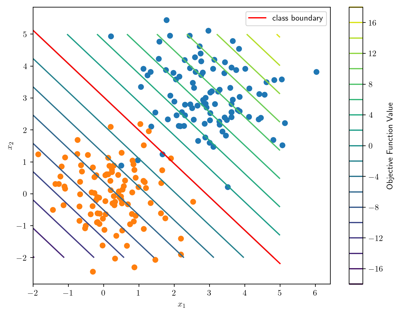
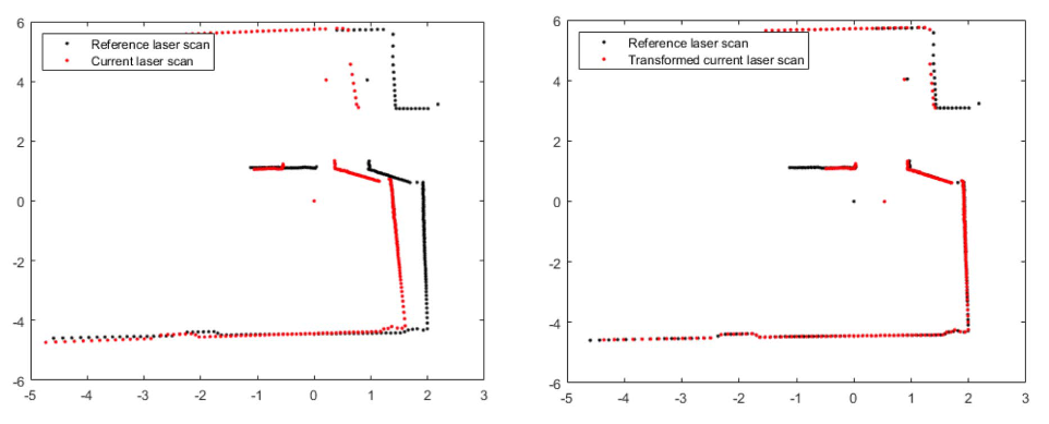
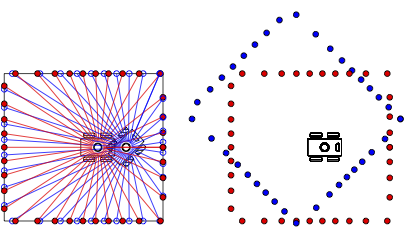
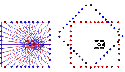
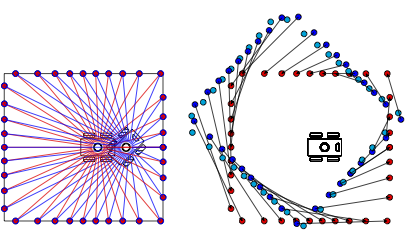
Laser scan taken at two different positions can be aligned to estimate robot motion
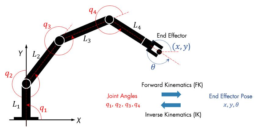
Given joint angles we can predict the end effector pose
Since we know how to build , we arrive at two approaches to inverse kinematics
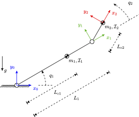
Frame has pose given by
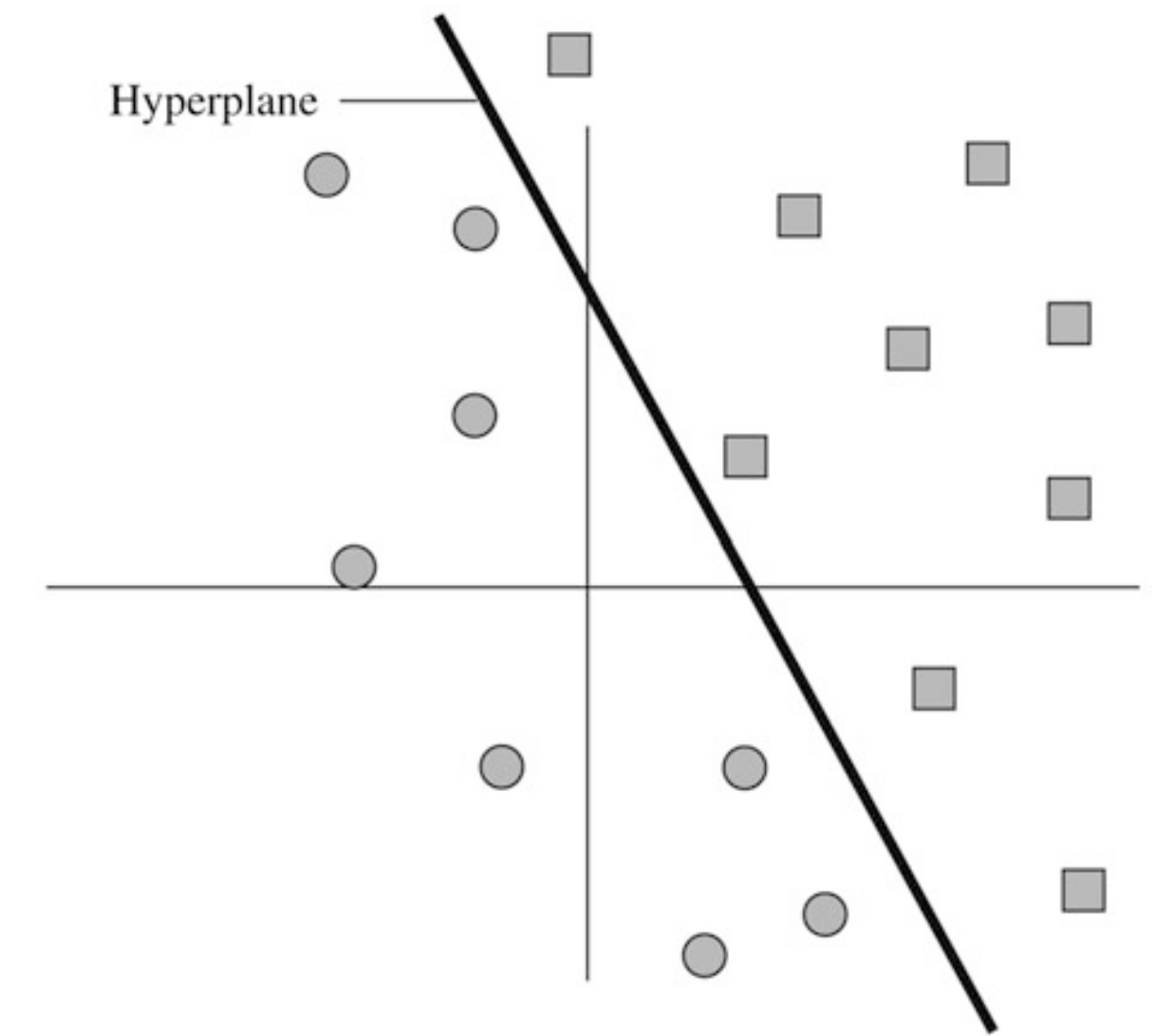
Two clusters of points (red) and (green) in (d=2)
We wish to classify the points into one of two clusters
We convert classification into regression by requiring that for some function :
One solution is to use the logistic function after linearly mapping inputs to a scalar:
New goal: find a vector and a number such that
which may equivalently be expressed using a log transformation as
Is this an easy or a hard problem?
The optimal value is 12.37578346960808
A solution x is
[2.35589697 2.25825204]
[-6.84717488]
# Import packages.
import cvxpy as cp
import numpy as np
import matplotlib.pyplot as plt
plt.rcParams['text.usetex'] = True
# Generate a random non-trivial linear program.
m = 100
n = 2
np.random.seed(1)
B = np.random.randn(m, n)
A = np.random.randn(m, n)+np.array([3,3])
plt.figure(figsize=(8, 6))
plt.scatter(A[:,0],A[:,1])
plt.scatter(B[:,0],B[:,1])
# beta = A @ x0 + s0
# c = -A.T @ lamb0
# Define and solve the CVXPY problem.
w = cp.Variable(n)
beta = cp.Variable(1)
prob = cp.Problem(cp.Minimize(cp.sum(cp.logistic( -A @ w- beta)) +cp.sum(cp.logistic( B @ w+ beta) ) ) )
# [A @ x <= beta])
prob.solve()
# Print result.
print("\nThe optimal value is", prob.value)
print("A solution x is")
print(w.value)
print(beta.value)
x = np.linspace(-2, 5, 100)
y = np.linspace(-2, 5, 100)
X, Y = np.meshgrid(x, y)
Z = (w.value[0]*X+w.value[1]*Y)+beta.value
# Contour plot of the objective function
contour = plt.contour(X, Y, Z, levels=20, cmap="viridis")
plt.colorbar(contour, label="Objective Function Value")
## Superimpose the line w^T x + beta = 0
x = np.linspace(-2, 5, 100)
y = -(w.value[0]/w.value[1])*x - beta.value/w.value[1]
plt.plot(x,y,color="red",label="class boundary")
plt.xlabel("$x_1$")
plt.ylabel("$x_2$")
plt.legend()
plt.show()
We solve the MDP by finding a policy that maximizes the expected discounted sum of rewards obtained from any state .
Through Dynamic Programming, we can solve for using the following Linear Program:
We seek to construct a cardboard box of maximum volume, given a fixed area of the cardboard.
First-Order Necessary Conditions
Since no variables can be zero, we have
A chain is suspended from two thin hooks that are ft. apart on a horizontal line. Each link is one foot in length (measured inside). We wish to formulate the problem to determine the equilibrium shape of the chain.
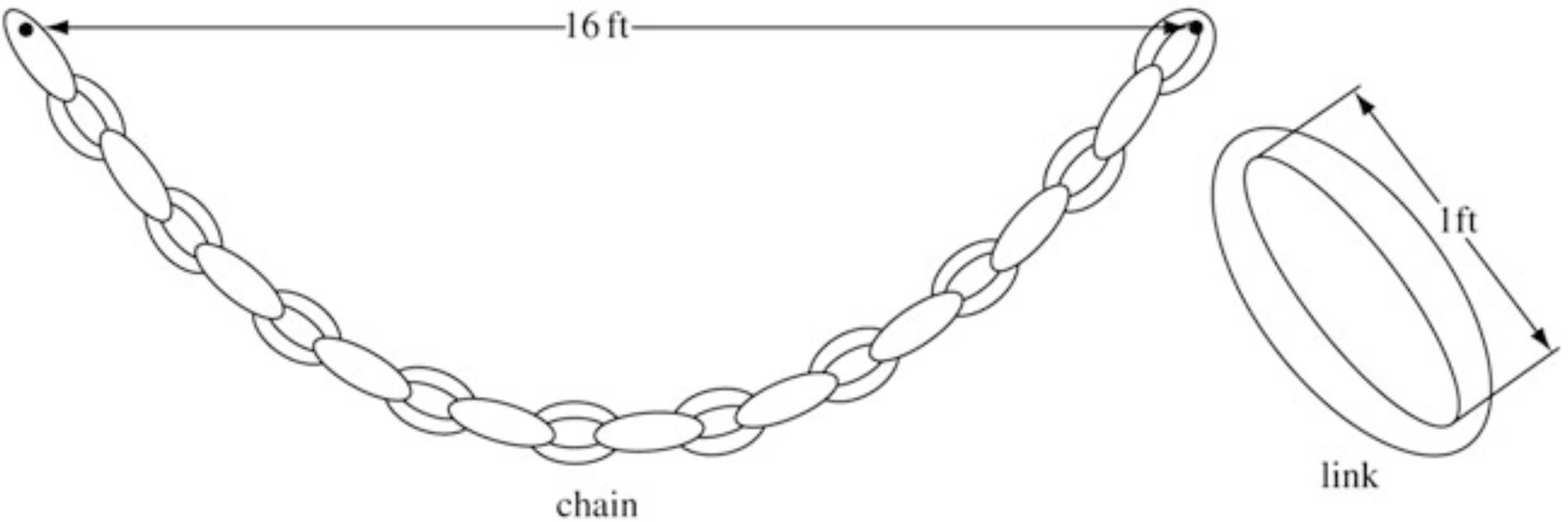
The solution can be found by minimizing the potential energy of the chain.
where in our example.
Constraints: The total displacement is zero and the total displacement is .
Formulation
First-Order Necessary Conditions
We want to solve the lienar equality constrained minimization problem.
The derivative of , when is .
Let us remove those zero entries in , then the remaining nonzero variables must still meet the FONC: for the column of and some
This means that the sum of the power of absolute values of the nonzero entries is bounded above. For , we have . Moreover,
Determine the most economical diet that satisfies the basic minimum nutritional requirements for good health
If we denote by the number of units of food in the diet, the problem is to select โs to minimize the total cost
subject to the nutritional constraints
and the nonnegative constraints on the food quantities.
This problem can be converted to standard form by subtracting a nonnegative surplus variable from the left side of each of the linear inequalities.
We wish to manufacture products at maximum revenue
subject to the resource constraints
and the nonnegativity consraints on all production variables.
| | |||||
| | |||||
| | |||||
| | |||||
โโ | โโ | โโ | โโ | ||
Maximal flow problem
Determine the maximal flow that can be established in such a network.
where for those no-arc pairs .
A warehouse is buying and selling stock of a certain commodity in order to maximize profit over a certain length of time.
where is a slack variable.
-dimensional data points are to be classified into two distinct classes.
where is the desired hyperplane.
Example
Systems Optimization I โข ME 647 Home