ME/AER 647 Systems Optimization I

---

Linear Programming

Instructor: Hasan A. Poonawala

Mechanical and Aerospace Engineering
University of Kentucky, Lexington, KY, USA

Topics:
Equality Constraints
Inequality Constraints
KKT Conditions

Introduction

Standard Form

Linear Program (LP)

An LP is an optimization problem in which the objective function is linear in the unknowns and the constraints consist of linear (in)equalities.

Standard form

$$\begin{align} \operatorname{minimize} & \bm{c}^\top \bm{x} = c_1x_1 + c_2x_2 + \cdots + c_nx_n \\ \text{subject to} & \bm{A}\bm{x} = \bm{b} \quad \text{and} \quad \bm{x} \geq \bm{0}. \end{align}$$

• $\bm{c}, \bm{x} \in \mathbb{R}^n$ are column vectors, $\bm{A} \in \mathbb{R}^{m \times n}$ a fat matrix ($m < n$), $\bm{b} \in \mathbb{R}^m$ a column vector.
• $b_i$’s, $c_i$’s and $a_{ij}$’s are fixed real constants, and the $x_i$’s are real numbers to be determined.
• We assume that each equation has been multiplied by minus unity, if necessary, so that each $b_i \geq 0$.

Conversion to Standard Form: Slack Variables

$$\begin{align} \operatorname{maximize} & c_1x_2 + c_2x_2 + \cdots + c_nx_n \\ \text{subject to} & a_{11}x_1 + a_{12}x_2 + \cdots + a_{1n}x_n &\leq b_1, \\ & a_{21}x_1 + a_{22}x_2 + \cdots + a_{2n}x_n &\leq b_2, \\ & \vdots & \vdots \\ & a_{m1}x_1 + a_{m2}x_2 + \cdots + a_{mn}x_n &\leq b_m, \\ & x_1, x_2, \ldots, x_n \geq 0. \end{align}$$

This problem may be alternatively expressed as

$$\begin{align} \operatorname{minimize} & -c_1x_2 - c_2x_2 - \cdots - c_nx_n \\ \text{subject to} & a_{11}x_1 + a_{12}x_2 + \cdots + a_{1n}x_n + x_{n+1} &= b_1, \\ & a_{21}x_1 + a_{22}x_2 + \cdots + a_{2n}x_n \phantom{12} + x_{n+2} &= b_2, \\ & \vdots & \vdots \\ & a_{m1}x_1 + a_{m2}x_2 + \cdots + a_{mn}x_n \phantom{12345} + x_{n+m} &= b_m, \\ & x_1, x_2, \ldots, x_{n+1}, \ldots, x_{n+m} \geq 0. \end{align}$$

• The new nonnegative variables $x_{n+i}$, $i=1, \ldots, m$ convert inequalities to equalities are called slack variables.

 

• The constrant matrix now is transformed to $\bm{A} \rightarrow \begin{bmatrix} \bm{A} & \bm{I} \end{bmatrix}$.

Conversion to Standard Form: Surplus Variables

• If the linear equalities are reversed so that a typical inequality is

$$a_{i1}x_1 + a_{i2}x_2 + \cdots + a_{in} x_n \geq b_i,$$

it is clear that this is equivalent to

$$a_{i1}x_1 + a_{i2}x_2 + \cdots + a_{in} x_n - y_i = b_i,$$

with $y_i \geq 0$.

• Variables, such as $y_i$, adjoined in this fashion to convert a “greater than or equal to” inequality to equality are called surplus variables.

• By suitably multiplying by minus unity, and adjoining slack and surplus variables, any set of linear inequalities can be converted to standard form.

Conversion to Standard Form: Free variables – First Method

Suppose one or more of the unknown variables is not required to be nonnegative, say, $x_1 \geq 0$ is not present so that $x_1$ is free to take on either positive or negative values.

• We then write $x_1 = u_1 - v_1$, and require that $u_1, v_1 \geq 0$.
• We substitute $u_1 - v_1$ for $x_1$ everywhere.
• The problem is then expressed in terms of the $n+1$ variables $u_1, v_1, x_2, x_3, \ldots, x_n$.
• There is a certain degree of redundancy introduced in this technique since a constant added to $u_1$ and $v_1$ does not change $x_1$.
• Nevertheless, the simplex method can still be used to find the solution.

Conversion to Standard Form: Free variables – Second Method

• Take the same free variable situation, i.e, $x_1$ is free to take on positive or negative values.
• One can take any one of the $m$ equality constraints which has a nonzero coefficient for $x_1$, say, for example,

$$a_{i1}x_1 + a_{i2}x_2 + \cdots + a_{in}x_n = b_i,$$

where $a_{i1} \neq 0$.

• Then $x_1$ can be expressed as a linear combination of the other variables, plus a constant.
• This expression can be substituted everywhere for $x_1$ and we are led to a new problem of exactly the same form but expressed in terms of the variables $x_2, x_3, \ldots, x_n$ only.
• Furthermore, the $i^{\text{th}}$ equation, used to determine $x_1$ is now identically zero and it too can be eliminated.
• We obtain a linear program having $n-1$ variables and $m-1$ constraint equations.

Example – Specific Case

$$\begin{align} \operatorname{minimize} & x_1 + 3x_2 + 4x_3 \\ \text{subject to} & x_1 + 2x_2 + x_3 = 5, \\ & 2x_1 + 3x_2 + x_3 = 6, \\ & x_2, x_3 \geq 0. \end{align}$$

$x_1$ is free, so we can solve for it from the first constraint, obtaining

$$x_1 = 5 - 2x_2 - x_3. \qquad(1)$$

Substituting this into the objective and the second constraint, we obtain the equivalent problem

$$\begin{align} \operatorname{minimize} & x_2 + 3x_3 \\ \text{subject to}& x_2 + x_3 = 4, \\ & x_2, x_3 \geq 0. \end{align}$$

which is a problem in standard form.

After the smaller problem is solved (what is the answer?) the value for $x_1 = -3$ can be found from Equation 1.

Examples of Linear Programming Problems

Example 1 – The Diet Problem

Determine the most economical diet that satisfies the basic minimum nutritional requirements for good health

• There are available $n$ different foods.
• There are $m$ basic nutritional ingredients,
• Each unit of food $j$ contains $a_{ij}$ units of the $i^{\text{th}}$ nutrient.

• $j^{\text{th}}$ food sells at a price $c_j$ per unit.
• Each individual must receive at least $b_i$ units of the $i^{\text{th}}$ nutrient per day.

If we denote by $x_j$ the number of units of food $j$ in the diet, the problem is to select $x_j$’s to minimize the total cost $$c_1x_1 + c_2x_2 + \cdots + c_nx_n$$

subject to the nutritional constraints $$a_{i1}x_1 + a_{i2}x_2 + \cdots + a_{in}x_n \geq b_i, \; i=1, \ldots, m,$$

and the nonnegative constraints $$x_1 \geq 0, x_2 \geq 0, \ldots, x_n \geq 0,$$ on the food quantities.

This problem can be converted to standard form by subtracting a nonnegative surplus variable from the left side of each of the $m$ linear inequalities.

Example 2– The Resource-Allocation Problem

• A facility is capable of manufacturing $n$ different products.
• Each product can be produced at any level $x_j \geq 0$, $j=1, 2, \ldots, n$.
• Each unit of the $j^{\text{th}}$ product needs $a_{ij}$ units of the $i^{\text{th}}$ resource, $i = 1, 2, \ldots, m$.

• Each product may require various amounts of $m$ different resources.
• Each unit of the $j^{\text{th}}$ product can sell for $\pi_j$ dollars.
• Each $b_i$, $i = 1, 2, \ldots, m$ describe the available quantities of the $m$ resources.

We wish to manufacture products at maximum revenue

$$\begin{align} \operatorname{maximize} & \pi_1x_1 + \pi_2x_2 + \cdots + \pi_nx_n \end{align}$$

subject to the resource constraints

$$\begin{align} \text{subject to} & a_{i1}x_1 + a_{i2}x_2 + \cdots + a_{in}x_n \leq b_i, \; i=1, \ldots, m \end{align}$$

and the nonnegativity consraints on all production variables.

• The problem can also be interpreted as
  • fund $n$ different activities, where
  • $\pi_j$ is the full reward from the $j^{\text{th}}$ activity,
  • $x_j$ is restricted to $0 \leq x_j \leq 1$, representing the funding level from $0\%$ to $100\%$.

Example 3 – The Transportation Problem

• Quantities $a_1, a_2, \ldots, a_m$ of a certain product are to be shipped from $m$ locations.
• Shipping a unit of product from origin $i$ to destination $j$ costs $c_{ij}$.

• These products will be received in amounts of $b_1, b_2, \ldots, b_n$ at each of $n$ destinations.
• We want to determine the amounts $x_{ij}$ to be shipped between each origin-destination pair $i = 1, 2, \ldots, m$; $j=1, 2, \ldots, n$.

$x_{11}$	$x_{12}$	$\cdots$	$x_{1n}$	|	$a_1$
$x_{21}$	$x_{22}$	$\cdots$	$x_{2n}$	|	$a_2$
$\vdots$	$\vdots$	$\vdots$	$\vdots$	|	$\vdots$
$x_{m1}$	$x_{m2}$	$\cdots$	$x_{mn}$	|	$a_m$
——	——	——	——
$b_{1}$	$b_{2}$	$\cdots$	$b_{n}$

• The $i^{\text{th}}$ row in this array defines the variables associated with the $i^{\text{th}}$ origin.
• The $j^{\text{th}}$ column defines the variables associated with the $j^{\text{th}}$ destination.
• Problem: find the nonnegative variables $x_{ij}$ so that the sum across the $i^{\text{th}}$ row is $a_j$, the sum down the $j^{\text{th}}$ column is $b_j$, and the weighted sum $\sum_{j=1}^n\sum_{i=1}^m c_{ij}x_{ij}$ is minimized.

Example 4 – The Maximal Flow Problem

Maximal flow problem

Determine the maximal flow that can be established in such a network.

$$\begin{align} \operatorname{maximize} & f \\ \text{subject to} & \sum_{j=1}^n x_{1j} - \sum_{j=1}^n x_{j1} - f = 0, \\ & \sum_{j=1}^n x_{ij} - \sum_{j=1}^n x_{ji} = 0, \quad i \neq 1, m, \\ & \sum_{j=1}^n x_{mj} - \sum_{j=1}^n x_{jm} + f = 0, \\ & 0 \leq x_{ij} \leq k_{ij}, \quad \forall i, j, \end{align}$$

where $k_{ij} = 0$ for those no-arc pairs $(i,j)$.

• Capacitated network in which two special nodes, called the source (node 1); and the sink (node $m$) are distinguished.
• All other nodes must satisfy the conservation requirement: net flow into these nodes must be zero.
  • the source may have a net outflow,
  • the sink may have a net inflow.
• The outlow $f$ of the source will equal the inflow of the sink.

Example 5 – A Supply-Chain Problem

A warehouse is buying and selling stock of a certain commodity in order to maximize profit over a certain length of time.

• Warehouse has a fixed capacity $C$.
• The price, $p_i$, of the commodity is known to fluctuate over a number of time periods, say months, indexed by $i$.
• The warehouse is originally empty and is required to be empty at the end of the last period.

• There is a cost $r$ per unit of holding stock for one period.
• In any period the same price holds for both purchase and sale.
• $x_i$: level of stock in the warehouse at the beginning of period $i$, $u_i$: amount bought during this period, $s_i$: amount sold during this period.

$$\begin{align} \operatorname{maximize} & \sum_{i=1}^n \left(p_i(s_i - u_i) - rx_i \right) \\ \text{subject to} & x_{i+1} = x_i + u_i - s_i, \quad i = 1, 2, \ldots, n-1, \\ & 0 = x_n + u_n - s_n, \\ & x_i + z_i = C, \quad i = 2, \ldots, n, \\ & x_1 = 0, x_i \geq 0, u_i \geq 0, s_i \geq 0, z_i \geq 0, \end{align}$$

where $z_i$ is a slack variable.

Example 6 – Linear Classifier and Support Vector Machine

$d$-dimensional data points are to be classified into two distinct classes.

• In general, we have vectors $\bm{a}_i \in \mathbb{R}^d$ for $i=1, 2, \ldots, n_1$ and vector $\bm{b}_j \in \mathbb{R}^d$ for $j = 1, 2, \ldots, n_2$.
• We wish to find a hyperplane that separates $\bm{a}_i$’s from the $\bm{b}_j$’s, i.e., find a slope-vector $y \in \mathbb{R}^d$ and an intercept $\beta$ such that

$$\begin{align} \bm{a}_i^\top \bm{y} + \beta &\geq 1, \quad \forall i, \\ \bm{b}_j^\top \bm{y} + \beta &\leq 1, \quad \forall j, \\ \end{align}$$

where $\{\bm{x}: \bm{x}^\bm{y} + \beta = 0\}$ is the desired hyperplane.

• The separation is defined by the fixed margins $+1$ and $-1$, which could be made soft or variable later.

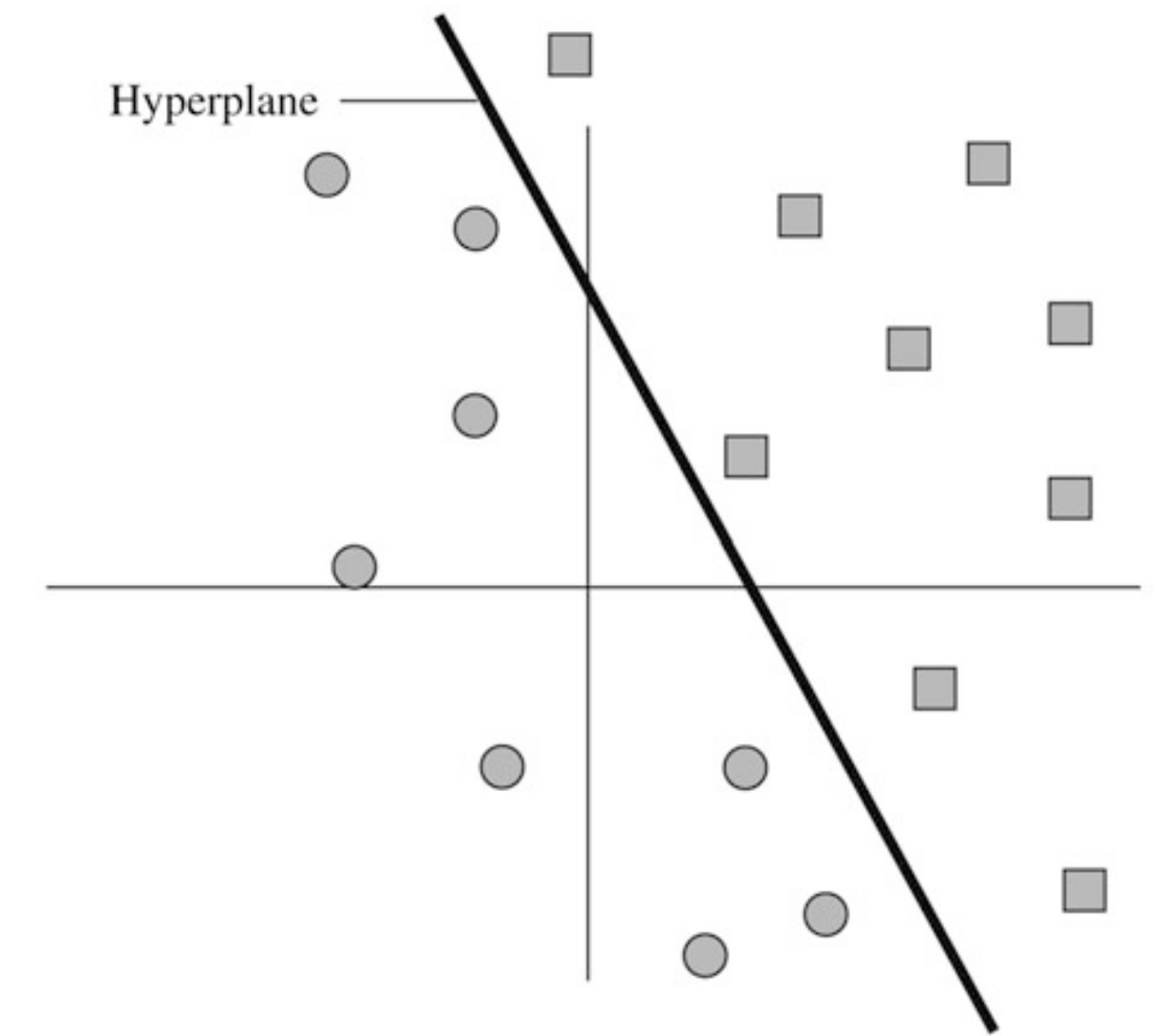
Example

• Two-dimensional data points may be grade averages in science and humanities for different students.
• We also know the academic major of each student, as being science or humanities, which serves as the classification.

Example 7 – Markov Decision Process (MDP)

Markov Decision Process

An MDP problem is defined by a finite number of states, indexed by $i = 1, \ldots, m$, where each state has a set of a finite number of actions, $\mathcal{A}_i$, to take.

• Each action, say $j \in \mathcal{A}_i$, is associated with
  • an immediate cost $c_j$ of taking,
  • a probability distribution $\bm{p}_j \in \mathbb{R}^m$ to transfer to all possible states at the next time period.
• A stationary policy for the decision maker is a function $\pi = \{\pi_1, \pi_2, \cdots, \pi_m\}$ that specifies a single action in every state, $\pi_i \in \mathcal{A}_i$.

MDP Problem

Find a stationary policy to minimize or maximize the discounted sum of expected costs or rewards over the infinite time horizon with a discount factor $0 \leq \gamma < 1$, when the process starts from state $i^0$:

$$\sum_{t=0}^\infty \gamma^t \mathbb{E}[c_{\pi_{i^t}}]$$

Example 7 – Markov Decision Process (MDP)

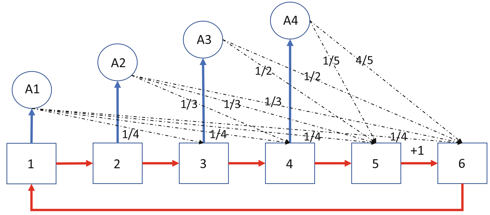
Maze Runner Game

Each square represents a state, where each of states $\{1, 2, 3, 4\}$ has two possible actions to take:

• red action: moves to the next state at the next time period,
• blue action: shortcut move, with a probability distribution, to a state at the next time period.

Each state of $\{5, 6\}$ has only one action

• moving to state $6$ (Exit state),
• moving to state $1$ (Start state).

All actions have zero cost, except state $5$’s (Trap state) action, which has a $1$-unit cost to get out.

Suppose that the game is played infinitely, what is the optimal policy? That is, which action is best to take for every state at any time, to minimize the present-expected total cost?

MDP Problem

Two constraints for the two actions of State $1$

$$y_1 - \gamma y_2 \leq 0, \;\; y_1 - \gamma(\frac{1}{4}y_3 + \frac{1}{4}y_5 + \frac{1}{4}y_6) \leq 0.$$

Only constraint for the single action of State $5$

$$y_5 - \gamma y_6 \leq 1.$$

Example 7 – Markov Decision Process (MDP)

• Let $y_i^\ast$, $i = 1, \ldots, m$ represent the optimal present-expected cost when the process starts at state $i$ and time $0$
  • also called the cost-to-go value of state $i$.
  • The $y_i^\ast$’s follow Bellman’s principle of optimality:

$$y_i^\ast = \operatorname{min}_{j \in \mathcal{A}_i} (c_j + \gamma \bm{p}_j^\top \bm{y}^\ast),$$

where $c_j$ is the immediate cost of taking action $j \in \mathcal{A}_i$ at the current time period, and $\bm{p}_j^\top \bm{y}^\ast$ is the optimal expected cost from the next time period, and then on.

• When $y_i^\ast$ is known for every state, the optimal action in each state would be

$$\pi_i^\ast = \operatorname{arg min}_{j \in \mathcal{A}_i} (c_j + \gamma \bm{p}_j^\top \bm{y}^\ast), \quad \forall i.$$

Example 7 – Markov Decision Process (MDP)

• One observes that $\bm{y}^\ast \in \mathbb{R}^m$ is a fixed-point of the Bellman operator, and it can be computed by the following linear program.

$$\begin{align} \operatorname{maximize} & \sum_{i=1}^m y_i \\ \text{subject to} & y_1 - \gamma \bm{p}_j^\top \bm{y} \leq c_j \quad \forall j \in \mathcal{A}_1, \\ & \vdots \\ & y_i - \gamma \bm{p}_j^\top \bm{y} \leq c_j \quad \forall j \in \mathcal{A}_i, \\ & \vdots \\ & y_m - \gamma \bm{p}_j^\top \bm{y} \leq c_j \quad \forall j \in \mathcal{A}_m. \\ \end{align}$$

• Basically, we relax the “$\operatorname{min}$” operator to “$\leq$” from Bellman’s principle and make them into the constraints and then maximize the sum of $y_i$’s as the objective.

• When the objective is maximized, at least one ineqality constraint in $\mathcal{A}_i$ must become equal for every state $i$ so that $\bm{y}$ is a fixed point solution of the Bellman operator.

Basic Feasible Solutions

Basic Solutions

System of equalities

$$\bm{Ax} = \bm{b} \qquad(2)$$

• From the $n$ columns of $\bm{A}$, we select a set of $m$ linearly independent columns.
• WLOG, assume that the first $m$ columns of $\bm{A}$ are selected: denote the $m \times m$ matrix determined by these columns by $\bm{B}$.
• The matrix $\bm{B}$ is nonsingular and we may uniquely solve the equation $$\bm{Bx_B} = \bm{b} \quad \text{or} \quad \bm{x_B} = \bm{B}^{-1}\bm{b}$$

• We refer to $\bm{B}$ as a basis, since $\bm{B}$ consists of $m$ linearly independent columns that can be regarded as a basis for $\mathbb{R}^m$.

Definition

Given the set of $m$ simultaneous linear equations $n$ unknowns Equation 2, let $\bm{B}$ be any nonsingular $m \times m$ submatrix made up of columns of $\bm{A}$. Then, if all $n-m$ components of $\bm{x}$ not associated with columns of $\bm{B}$ are set equal to zero, the solution to the resulting set of equations is said to be a basic solution to Equation 2 with respect to basis $\bm{B}$.

Definition

The components of $\bm{x}$ associated with the columns of $\bm{B}$, denoted by the subvector $\bm{x}_B$ according to the same column index order in $\bm{B}$, are called basic variables.

Full-Rank Assumption

The $m \times n$ matrix $\bm{A}$ has $m < n$, and the $m$ rows of $\bm{A}$ are linearly independent.

Basic Feasible Solutions

Definition

If one or more of the basic variables in a basic solution has value zero, that solution is said to be a degenerate basic solution.

• In a nondegenerate basic solution, the basic variables, and hence the basis $\bm{B}$, can be immediately identified from the positive components of the solution.
  • There is ambiguity associated with a degenerate basic solution – some of the nonbasic variables can be interchanged!

Definition

A vector $\bm{x}$ satisfying

$$\bm{Ax} = \bm{b}, \quad \bm{x} \geq \bm{0}, \qquad(3)$$

is said to be feasible for these constraints. A feasible solution to the constraints Equation 3 that is also basic is said to be a basic feasible solution; if this solution is also a degenerate basic solution, it is called a degenerate basic feasible solution.

The Fundamental Theorem of Linear Programming

The Fundamental Theorem of LP

Corresponding to a linear program in standard form

$$\begin{align} \operatorname{minimize} & \bm{c}^\top \bm{x} \\ \text{subject to} & \bm{Ax} = \bm{b}, \;\; \bm{x} \geq 0 \end{align} \qquad(4)$$

a feasible solution to the constraints that achieves the minimum value of the objective function subject to those constraints is said to be an optimal feasible solution. If this solution is basic, it is an optimal basic feasible solution.

Fundamental Theorem

Given a linear program in standard form Equation 4 where $\bm{A}$ is an $m \times n$ matrix of rank $m$,

1. if there is a feasible solution, there is a basic feasible solution;
2. if there is an optimal feasible solution, there is an optimal basic feasible solution.

Proof (1)

Denote the columns of $\bm{A}$ by $\bm{a}_1, \bm{a}_2, \ldots, \bm{a}_n$. Suppose $\bm{x} = (x_1, x_2, \ldots, x_n)$ is a feasible solution. Then, in terms of the columns of $\bm{A}$, this solution satisfies

$$x_1\bm{a}_1 + x_2\bm{a}_2 + \cdots + x_n\bm{a}_n = \bm{b}.$$

The Fundamental Theorem of LP

Proof (1) - Continued -

Assume that exactly $p$ of the variables $x_i$ are greater than zero, and wlog, that they are the first $p$ variables. Thus

$$x_1 \bm{a}_1 + x_2 \bm{a}_2 + \cdots + x_p \bm{a}_p = \bm{b}. \qquad(5)$$

There are now two cases, corresponding as to whether the set $\bm{a}_1, \bm{a}_2, \ldots, \bm{a}_p$ is linearly independent or linearly dependent.

Case 1: Assume $\bm{a}_1, \bm{a}_2, \ldots, \bm{a}_p$ are linearly independent. Then clearly, $p \leq m$. If $p = m$, the solution is basic and the proof is complete. If $p < m$, then, since $\bm{A}$ has rank $m$, $m-p$ vectors can be found from the remaining $n-p$ vectors so that the resulting set of $m$ vectors is linearly independent. Assigning the value zero to the corresponding $m-p$ variables yields a (degenerate) basic feasible solution.

Case 2: Assume $\bm{a}_1, \bm{a}_2, \ldots, \bm{a}_p$ are linearly dependent. Then there is a nontrivial linear combination of these vectors that is zero. Thus there are constants $y_1, y_2, \ldots, y_p$, at least one of which can be assumed to be positive, such that

$$y_1\bm{a}_1 + y_2\bm{a}_2 + \cdots + y_p\bm{a}_p = \bm{0}. \qquad(6)$$

Multiplying this equation by a scalar $\varepsilon$ and subtracting it from Equation 5, we obtain

$$(x_1 - \varepsilon y_1)\bm{a}_1 + (x_2 - \varepsilon y_2)\bm{a}_2 + \cdots + (x_p - \varepsilon y_p)\bm{a}_p = \bm{b}. \qquad(7)$$

This equation holds for every $\varepsilon$, and for each $\varepsilon$ the components $x_j - \varepsilon y_j$ correspond to a solution of the linear equalities — although they may violate $x_i - \varepsilon y_i \geq 0$. Denoting $\bm{y} = (y_1, y_2, \ldots, y_p, 0, 0, \ldots, 0)$, we see that for any $\varepsilon$

$$\bm{x} - \varepsilon \bm{y} \qquad(8)$$

is a solution to the equalities. For $\varepsilon = 0$, this reduces to the original feasible solution.

The Fundamental Theorem of LP

Proof (1) - Continued -

As $\varepsilon$ is increased from zero, the various components increase, decrease, or remain constant, depending upon whether the correspoding $y_i$ is negative, positive, or zero. Since we assume at least one $y_i$ is positive, at least one component will decrease as $\varepsilon$ is increased. we increase $\varepsilon$ to the first point where one or more components become zero. Specifically, we set

$$\varepsilon = \operatorname{min}\left\{\frac{x_i}{y_i}: y_i > 0 \right\}.$$

For this value of $\varepsilon$, the solution given by Equation 8 is feasible and has at most $p-1$ positive variables. Repeating this process as necessary, we can eliminate positive variables until we have a feasible solution with corresponding columns that are linearly independent. At that point Case 1 applies.

Proof (2)

Let $\bm{x} = (x_1, x_2, \ldots, x_n)$ be an optimal feasible solution and, as in the proof of (1) above, suppose there are exactly $p$ positive variables $x_1, x_2, \ldots, x_p$. Again, there are two cases; and Case 1, corresponding to the linear independence is exactly the same as before.

Case 2 also goes exactly the same as before, but it must be shown that for any $\varepsilon$ the solution Equation 8 is optimal. To show this, note that the value of the solution $\bm{x} - \varepsilon\bm{y}$ is

$$\bm{c}^\top \bm{x} - \varepsilon \bm{c}^\top \bm{y}. \qquad(9)$$

For $\varepsilon$ sufficiently small in magnitude, $\bm{x} - \varepsilon \bm{y}$ is a feasible solution for positive or negative values of $\varepsilon$. Thus, we conclude that $\bm{c}^\top \bm{y} = \bm{0}$ (why?).

Proof (2)

Let $\bm{x} = (x_1, x_2, \ldots, x_n)$ be an optimal feasible solution and, as in the proof of (1) above, suppose there are exactly $p$ positive variables $x_1, x_2, \ldots, x_p$. Again, there are two cases; and Case 1, corresponding to the linear independence is exactly the same as before.

Case 2 also goes exactly the same as before, but it must be shown that for any $\varepsilon$ the solution Equation 8 is optimal. To show this, note that the value of the solution $\bm{x} - \varepsilon\bm{y}$ is

$$\bm{c}^\top \bm{x} - \varepsilon \bm{c}^\top \bm{y}. \qquad(10)$$

For $\varepsilon$ sufficiently small in magnitude, $\bm{x} - \varepsilon \bm{y}$ is a feasible solution for positive or negative values of $\varepsilon$. Thus, we conclude that $\bm{c}^\top \bm{y} = \bm{0}$. For, if $\bm{c}^\top \bm{y} \neq \bm{0}$, an $\varepsilon$ of small magnitude and proper sign could be determined so as to render Equation 10 smaller than $\bm{c}^\top \bm{y}$ while maintaining feasibility.

The Fundamental Theorem of LP

• Part (1) of the theorem is commonly referred to as Carathéodory’s theorem.

• Part (2) of the theorem reduces the task of solving a linear program to that of searching over basic feasible solutions.

• Since for a problem having $n$ variables and $m$ constraints there are at most

$$\binom{n}{m} = \frac{n!}{m!(n-m)!}$$

basic solutions (corresponding to the number of ways of selecting $m$ of $n$ columns), there are only a finite number of possibilities.

• Thus the fundamental theorem yields an obvious, but terribly inefficient, finite search technique.

• By expanding upon the technique of proof as well as the statement of the fundamental theorem, the efficient simplex procedure is derived.

Relations to Convex Geometry

Extreme Points

Definition

A point $\bm{x}$ in a convex set $C$ is said to be an extreme point of $C$ if there are no two distinct points $\bm{x}_1$ and $\bm{x}_2$ in $C$ such that $\bm{x} = \alpha \bm{x}_1 + (1-\alpha)\bm{x}_2$ for some $\alpha$, $0 < \alpha < 1$.

• An extreme point is thus a point that does not lie strictly within a line segment connecting two other points of the set.

Theorem (Equivalence of Extreme Points and Basic Solutions).

Let $\bm{A}$ be an $m \times n$ matrix of rank $m$ and $\bm{b}$ an $m$-vector. Let $K$ be the convex polytope consisting of all $n$-vectors $\bm{x}$ satisfying

$$\bm{Ax} = \bm{b}, \;\; \bm{x} \geq \bm{0}. \qquad(11)$$

A vector $\bm{x}$ is an extreme point of $K$ if and only if $\bm{x}$ is a basic feasible solution to Equation 11.

Proof

Suppose first that $\bm{x} = (x_1, x_2, \ldots, x_m, 0, 0, \ldots, 0)$ is a basic feasible solution to Equation 11. Then

$$x_1 \bm{a}_1 + x_2\bm{a}_2 + \cdots + x_m\bm{a}_m = \bm{b},$$

where $\bm{a}_1, \bm{a}_2, \ldots, \bm{a}_m$, the first $m$ columns of $\bm{A}$ are linearly independent. Suppose that $\bm{x}$ could be expressed as a convex combination of two other points in K; say, $\bm{x} = \alpha \bm{y} + (1-\alpha)\bm{z}$, $0 < \alpha < 1$, $\bm{y} \neq \bm{z}$.

Extreme Points

Proof

Since all components of $\bm{x}$, $\bm{y}$, $\bm{z}$ are nonnegative and since $0 < \alpha < 1$, it follows immediately that the last $n-m$ components of $\bm{y}$ and $\bm{z}$ are zero. Thus, in particular, we have

$$y_1\bm{a}_1 + y_2\bm{a}_2 + \cdots + y_m\bm{a}_m = \bm{b}$$

and

$$z_1\bm{a}_1 + z_2\bm{a}_2 + \cdots + z_m\bm{a}_m = \bm{b}.$$

Since the vectors $\bm{a}_1, \bm{a}_2, \ldots, \bm{a}_m$ are linearly independent, however, it follows that $\bm{x} = \bm{y} = \bm{z}$ and hence $x$ is an extreme point of $K$.

Conversely, assume that $\bm{x}$ is an extreme point of $K$. Let us assume that the nonzero components of $\bm{x}$ are the first $k$ components. Then

$$x_1\bm{a}_1 + x_2\bm{a}_2 + \cdots + x_k\bm{a}_k = \bm{b}, \quad x_i > 0, \quad i = 1, 2, \ldots, k.$$

To show that $\bm{x}$ is a basic feasible solution (BFS) it must be shown that the vectors $\bm{a}_1, \bm{a}_2, \ldots, \bm{a}_k$ are linearly independent. We do this by contradiction. Suppose they are linearly dependent. Then there is a nontrivial linear combination that is zero:

$$y_1\bm{a}_1 + y_2\bm{a}_2 + \cdots y_k\bm{a}_k = \bm{0}.$$

Define the $n$-vector $\bm{y} = (y_1, y_2, \ldots, y_k, 0, 0, \ldots, 0)$. Since $x_i > 0$, $1 \leq i \leq k$, it is possible to select $\varepsilon$ such that

$$\bm{x} + \varepsilon \bm{y} \geq \bm{0}, \quad \bm{x} - \varepsilon \bm{y} \geq \bm{0}.$$

We then have $\bm{x} = \frac{1}{2}(\bm{x}+\varepsilon\bm{y}) + \frac{1}{2}(\bm{x}-\varepsilon\bm{y})$ which expresses $\bm{x}$ as a convex combination of two distinct vectors in $K$.

Extreme Points

Corollary

If the convex set $K$ corresponding to Equation 11 is nonempty, it has at least one extreme point.

Corollary

If there is a finite optimal solution to a linear programming problem, there is a finite optimal solution which is an extreme point of the constraint set.

Corollary

The constraint set $K$ corresponding to Equation 11 possesses at most a finite number of extreme points and each of them is finite.

Corollary

If the convex polytope $K$ corresponding to Equation 11 is bounded, then $K$ is a convex polyhedron, that is, $K$ consists of points that are convex combinations of a finite number of points.

Convex Geometry – Examples

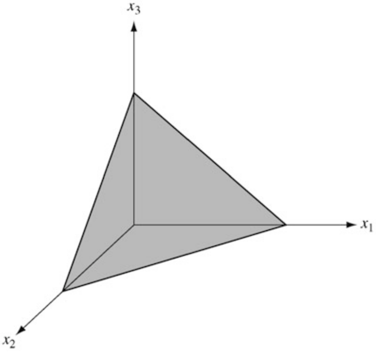
Consider the constraint set in $\mathbb{R}^3$ defined by

$$\begin{align} x_1 + x_2 + x_3 &= 1, \\ x_1, x_2, x_3 &\geq 0. \end{align}$$

• This set is illustrated in the figure.
• It has three extreme points, corresponding to the three basic solutions to $x_1 + x_2 + x_3 = 1$.

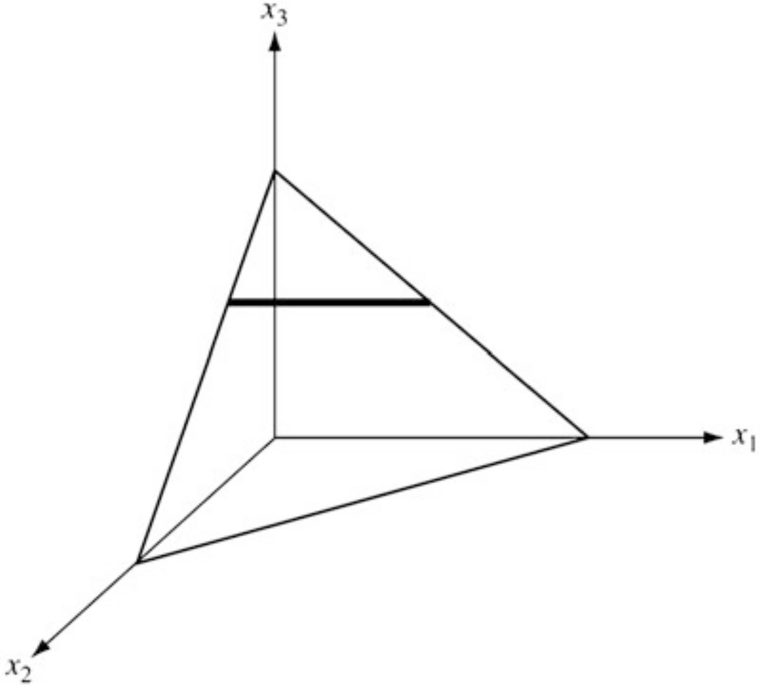
Consider the constraint set in $\mathbb{R}^3$ defined by

$$\begin{align} x_1 + x_2 + x_3 &= 1, \\ 2x_1 + 3x_2 &= 1, \\ x_1, x_2, x_3 &\geq 0. \end{align}$$

• This set is illustrated in the figure.
• It has two extreme points, corresponding to the two basic feasible solutions.
• Note that the system of equations itself has three basic solutions: $$(2, -1, 0), (\frac{1}{2}, 0, \frac{1}{2}), (0, \frac{1}{3}, \frac{2}{3}),$$ the first of which is not feasible.

Convex Geometry – Examples

Consider the constraint set in $\mathbb{R}^2$ defined by

$$\begin{align} x_1 + \frac{8}{3}x_2 &\leq 4, \\ x_1 + x_2 &\leq 2, \\ 2x_1 &\leq 3, \\ x_1, x_2 &\geq 0. \end{align}$$

• The set has five extreme points.
• In order to compare this example, we must introduce slack variables to yield the equivalent set in $\mathbb{R}^5$.

$$\begin{align} x_1 + \frac{8}{3}x_2 + x_3 &= 4, \\ x_1 + x_2 + x_4 &= 2, \\ 2_x1 + x_5 &= 3 \\ x_1, x_2, x_3, x_4, x_5 \geq 0. \end{align}$$

• A basic solution for this system is obtained by setting any two variables to zero and solving for the remaining three.

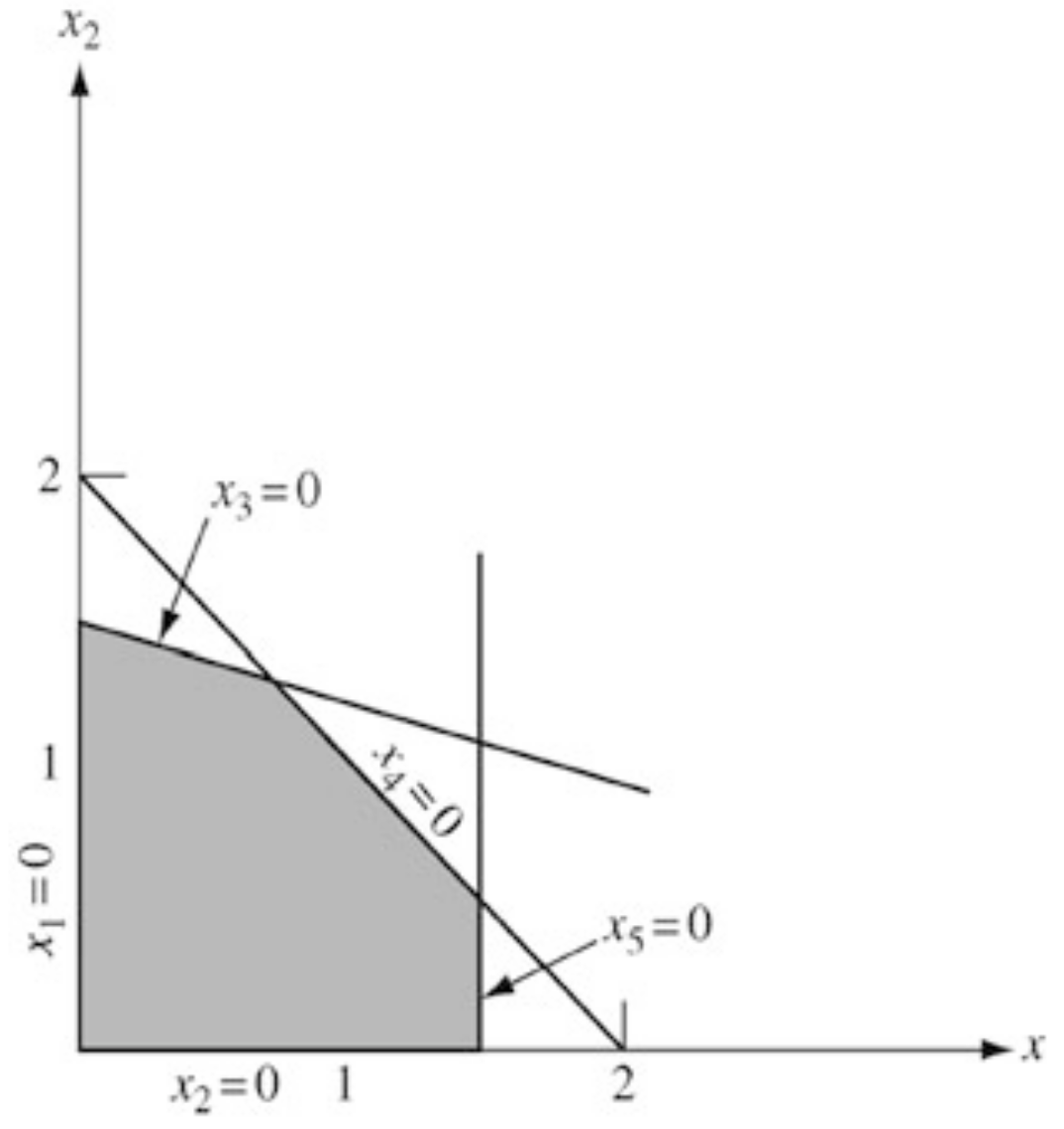
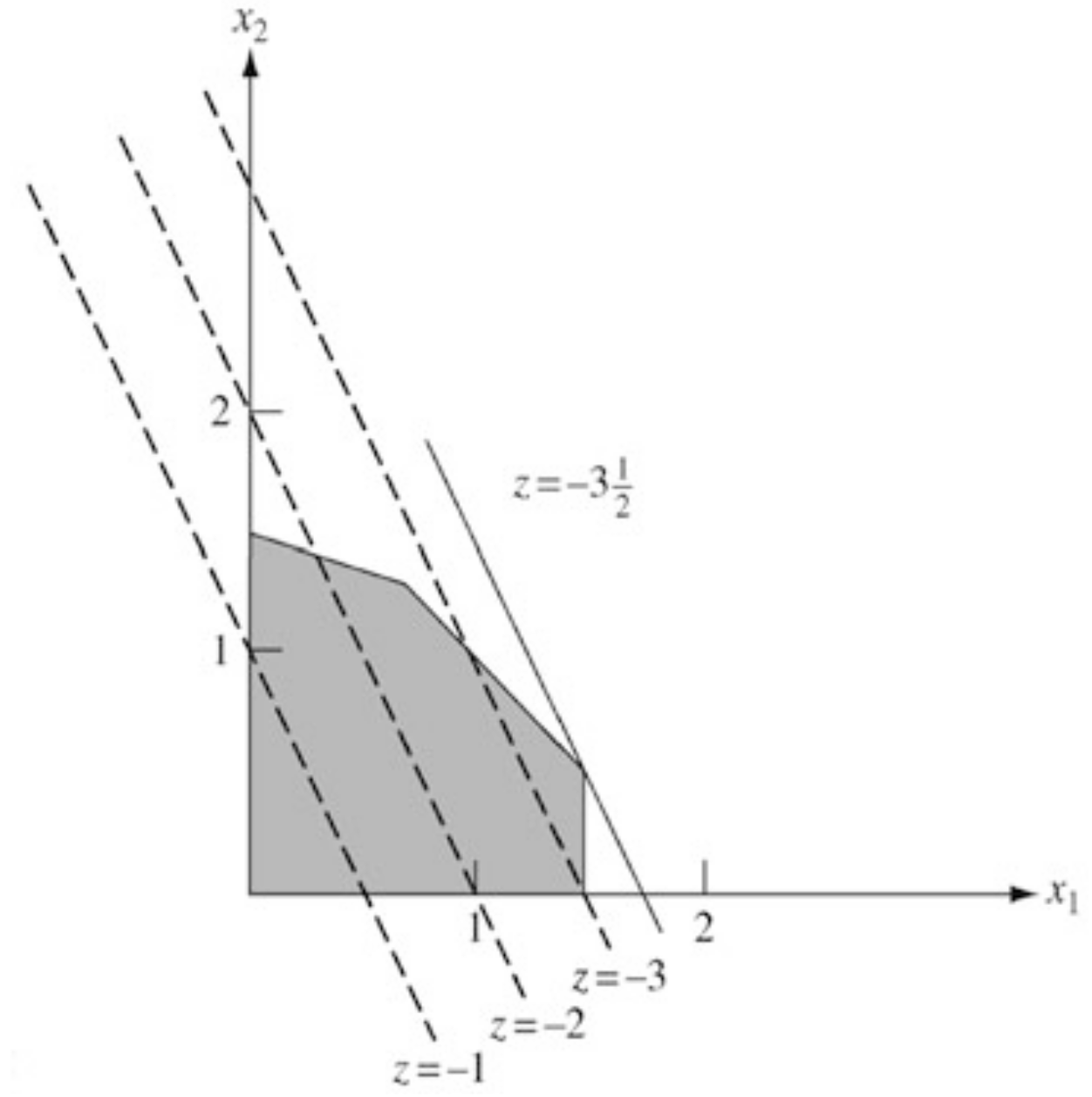
• A basic solution for this system is obtained by setting any two variables to zero and solving for the remaining three.

• As indicated in the figure, each edge of the figure corresponds to one variable being zero, and the extreme points are the points where two variables are zero.

• Even when not expressed in the standard form, the extreme points of the set defined by the constraints of a lienar program correspond to the possible solution points.

• The level sets of an objective function $-2x_1 - x_2$ is included in the bottom figure.

  • As the level varies, different parallel lines are obtained.
  • The optimal value of the linear program is the smallest value of this level for which the corresponding line has a point in common with the feasible set.
  • In the figure, this occurs at the point $(\frac{3}{2}, \frac{1}{2})$ with the level $z = -\frac{7}{2}$.

Farkas’s Lemma and Alternative Systems

(In)feasibility Certificates

Theorem (Farkas’s Lemma).

Let $\bm{A}$ be an $m \times n$ matrix and $\bm{b}$ be an $m$-vector. The system of constraints $$\bm{Ax} = \bm{b}, \quad \bm{x} \geq \bm{0} \qquad(12)$$ has a feasible solution $\bm{x}$ if and only if the system of constraints $$-\bm{y}^\top \bm{A} \geq \bm{0}, \quad \bm{y}^\top \bm{b} = 1 (\text{or} > 0) \qquad(13)$$ has no feasible solution $\bm{y}$. Therefore a single feasible solution $\bm{y}$ for system Equation 13 establishes an infeasibility certificate for the system Equation 12.

• The two systems, Equation 12 and Equation 13, are called alternative systems: one of them is feasible and the other is infeasible.

Example 1

Suppose $\bm{A} = \begin{bmatrix} 1 & 1 \end{bmatrix}, \quad \bm{b} = -1$. Then, $y = -1$ is feasible for system Equation 13, which proves that the system Equation 12 is infeasible.

(In)feasibility Certificates

Lemma

Let $C$ be the cone generated by the columns of matrix $\bm{A}$, that is $$C = \{\bm{Ax} \in \mathbb{R}^m: \bm{x} \geq \bm{0}\}.$$ Then C is a closed and convex set.

Proof (of Farkas’s Lemma).

Let the system Equation 12 have a feasible solution, say $\bar{\bm{x}}$. Then, the system Equation 13 must be infeasible, since, otherwise, we have a contradiction

$$0 < \bm{y}^\top \bm{b} = \bm{y}^\top(\bm{A}\bar{\bm{x}}) = (\bm{y}^\top \bm{A})\bar{\bm{x}} \leq 0,$$

from $\bar{\bm{x}} \geq \bm{0}$ and $\bm{y}^\top \bm{A} \leq \bm{0}$.

Now, let the system Equation 12 have no feasible solution, that is, $\bm{b} \notin C := \{\bm{Ax}: \bm{x} \geq 0\}$. We now prove that its alternative system Equation 13 must have a feasible solution.

Since points $\bm{b}$ is not in $C$ and $C$ is a closed convex set, by the separating hyperplane theorem, there is a $\bm{y}$ such that $$\bm{y}^\top \bm{b} > \operatorname{sup}_{\bm{c} \in C} \bm{y}^\top \bm{c}.$$ But we know that $\bm{c} = \bm{Ax}$ for some $\bm{x} \geq \bm{0}$, so we have $$\bm{y}^\top \bm{b} > \operatorname{sup}_{\bm{x}\geq\bm{0}} \bm{y}^\top \bm{Ax} = \operatorname{sup}_{\bm{x} \geq \bm{0}} (\bm{y}^\top \bm{A})\bm{x}. \qquad(14)$$ Setting $\bm{x} = \bm{0}$, we have $\bm{y}^\top \bm{b} > 0$ from inequality Equation 14.

(In)feasibility Certificates

Proof (of Farkas’s Lemma) - Continued -

Furthermore, inequality Equation 14 also implies $\bm{y}^\top \bm{A} \leq \bm{0}$. Since otherwise, say the first entry of $\bm{y}^\top \bm{A}$, $(\bm{y}^\top \bm{A})_1$, is positive. We can then choose a vector $\bar{\bm{x}} \geq \bm{0}$ such that

$$\bar{x}_1 = \alpha > 0, \bar{x}_2 = \cdots = \bar{x}_n = 0.$$

Then, from this choice, we have

$$\operatorname{sup}_{\bm{x} \geq \bm{0}} (\bm{y}^\top\bm{A})\bm{x} \geq (\bm{y}^\top \bm{A})\bar{\bm{x}} = \alpha(\bm{y}^\top \bm{A})_1.$$

This tends to $\infty$ as $\alpha \rightarrow \infty$. This is a contradiction because $(\bm{y}^\top\bm{A})\bar{\bm{x}}$ should be bounded from above by inequality Equation 14. Therefore, $\bm{y}$ identified in the separating hyperplane theorem is a feasible solution to system Equation 13. Finally, we can always scale $\bm{y}$ such that $\bm{y}^\top \bm{b} = 1$.

Geometric Interpretation

If $\bm{b}$ is not in the closed and convex cone generated by the columns of the matrix $\bm{A}$, then there must be a hyperplane separating $\bm{b}$ and the cone, and the feasible solution $\bm{y}$ to the alternative system is the slope-vector of the hyperplane.

Variant of Farkas’s Lemma

Corollary

Let $\bm{A}$ be an $m \times n$ matrix and $\bm{c}$ an $n$-vector. The system of constraints

$$\bm{A}^\top \bm{y} \leq c \qquad(15)$$

has a feasible solution $\bm{y}$ if and only if the system of constraints

$$\bm{Ax} = \bm{0}, \quad \bm{x} \geq \bm{0}, \quad \bm{c}^\top \bm{x} = -1 \; (\text{or} < 0) \qquad(16)$$

has no feasible solution $\bm{x}$. Therefore a single feasible solution $\bm{x}$ for system Equation 16 establishes an infeasibility certificate for the system Equation 15.

Adjacent Basic Feasible Solutions (Extreme Points)

Adjacent Solutions

• We know that it is only necessary to consider basic feasible solutions to the system $$\bm{Ax} = \bm{b}, \quad \bm{x} \geq \bm{0} \qquad(17)$$ when solving a linear program.

• The idea of the simplex method is to move from a basic feasible solution (extreme point) to an adjacent one with an improved objective value.

Definition

Two basic feasible solutions are said to be adjacent if and only if they differ by one basic variable.

• A new basic solution can be generated from an old one by replacing one current basic variable by a current nonbasic one.
  • It is impossible to arbitrarily specify a pair of variables whose roles are to be interchanged and expect to maintain the nonnegativity condition.
  • However, it is possible to arbitrarily specify which current nonbasic (entering or incoming) variable is to become basic and then determine which current basic (leaving or outgoing) variable should become nonbasic.

Determination of a Vector to Leave the Basis

• Let the BFS be partitioned as $\bm{x}_{\bm{B}} = (x_1, x_2, \ldots, x_m)$ and $\bm{x}_{\bm{D}} = (x_{m+1}, x_{m+2}, \ldots, x_n)$.

• $\bm{b}$ is a linear combination of columns of $\bm{B} = \begin{bmatrix} \bm{a}_1 & \bm{a}_2 & \cdots & \bm{a}_m \end{bmatrix}$ with the positive multipliers $(x_1, x_2, \ldots, x_m)$.

$$\bm{b} = \bm{B}\bm{x}_{\bm{B}} = x_1\bm{a}_1 + x_2 \bm{a}_2 + \cdots + x_m\bm{a}_m, \quad \text{where} \quad \bm{x}_{\bm{B}} = \bar{\bm{a}}_0 := \bm{B}^{-1}\bm{b} \geq \bm{0}. \qquad(18)$$

• Suppose we decided to bring into representation the $e^{\text{th}}$ (entering) column vector of $\bm{A}$, $\bm{a}_e$ ($e > m$), while keeping all others nonbasic.

• A new representation of $\bm{b}$ as a linear combination of $m+1$ vectors ($\bm{a}_e$ added to the current basis $\bm{B}$) for any nonnegative multiplier $x_e$ and $\bm{x}_{\bm{B}}$:

$$\bm{b} = \bm{Bx_B} + \bm{a}_ex_e, \quad \text{or} \quad \bar{\bm{a}}_0 = \bm{B}^{-1}\bm{b} = \bm{x}_{\bm{B}} + (\bm{B}^{-1}\bm{a}_e)x_e. \qquad(19)$$

• Since $x_e$ is the incoming variable, its value needs to be increased from the current $0$ to a positive value, say $\varepsilon \geq 0$.

• As $x_e$ value increases, the current basic variable $\bm{x}_{\bm{B}}$ needs to be adjusted accordingly to keep the feasibility.

$$\bm{x}_{\bm{B}} = \bar{\bm{a}}_0 - \varepsilon(\bm{B}^{-1}\bm{a}_e) = \bar{\bm{a}}_0 - \varepsilon\bar{\bm{a}}_e \geq \bm{0}, \quad \text{where} \quad \bar{\bm{a}}_e = \bm{B}^{-1}\bm{a}_e. \qquad(20)$$

Determination of a Vector to Leave the Basis

• For $\varepsilon = 0$, we have the old basic feasible solution $\bm{x}_{\bm{B}} = \bar{\bm{a}}_0 > \bm{0}$.
• The values of $\bm{x}_{\bm{B}}$ will either increase or remain unchanged if $\bar{a}_{ie} \leq 0$; or decrease linearly as $\varepsilon$ is increased if $\bar{a}_{ie} > 0$.

• For small enough $\varepsilon$, Equation 19 gives a feasible but nonbasic solution.
• If any decrease, we may set $\varepsilon$ equal to the value corresponding to the first place where one (or more) of the value vanishes

$$\varepsilon = \operatorname{min}_i \left\{\frac{\bar{a}_{i0}}{\bar{a}_{ie}}: \bar{a}_{ie} > 0 \right\}. \qquad(21)$$

• We have a new BFS, with the vector $\bm{a}_e$ replacing (outgoing) column $\bm{a}_o$, where index $o \leq m$ corresponds to the minimizing-ratio in Equation 21 $$o = \operatorname{arg \, min}_i \left\{\frac{\bar{a}_{i0}}{\bar{a}_{ie}}: \bar{a}_{ie} > 0 \right\}.$$

• If none of the $\bar{a}_{ie}$’s are positive, then all coefficients in Equation 19 increase (or remain constant) as $\varepsilon$ is increased, and no new basic feasible solution is obtained.

• In this case the set $K$ of feasible solutions to Equation 17 is unbounded.

Conic Combination Interpretations

• The basis transformation can be represented in the requirements space, the space where columns of $\bm{A}$ and $\bm{b}$ are represented.

$$\bm{a}_1x_1 + \bm{a}_2x_2 + \cdots + \bm{a}_nx_n = \bm{b}.$$

• A feasible solution defines a representation of $\bm{b}$ as a conic combination of the $\bm{a}_i$’s.
• A BFS will only use $m$ positive weights.
• Suppose we start with $\bm{a}_1$ and $\bm{a}_2$ as the initial basis.
  • Then an adjacent basis is found by bringing in some other vector.
  • If $\bm{a}_3$ is brought in, then clearly $\bm{a}_2$ must go out (why?).
  • On the other hand, if $\bm{a}_4$ is brought in, $\bm{a}_1$ must go out (why?).

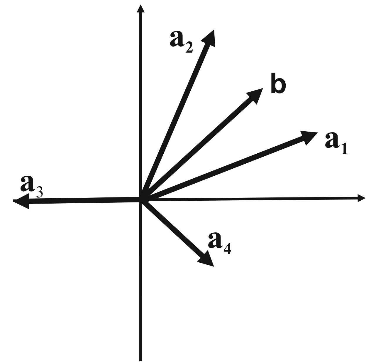
• A BFS can be constructed with positive weights on $\bm{a}_1$ and $\bm{a}_2$ because $\bm{b}$ lies between them.
• A BFS cannot be constructed with positive weights on $\bm{a}_1$ and $\bm{a}_4$.

• Another interpretation is in the activity space, the space where $\bm{x}$ lives.
  • Here, the feasible region is shown directly as a convex set, and BFS are extreme points.
  • Adjacent extreme points are points that lie on a common edge.

Conic Combination Interpretations – Example

Example (Basis Change Illustration)

$$\begin{align} 3x_1 + x_2 - 2x_3 + x_4 &= 2, \\ x_1 + 3x_2 - x_4 &= 2. \end{align}$$

• Suppose we start with $\bm{a}_1$ and $\bm{a}_2$ as the initial basis and select $\bm{a}_3$ as the incoming column. Then

$$\begin{equation} \bm{B} = \begin{pmatrix} 3 & 1 \\ 1 & 3 \end{pmatrix}, \quad \bm{B}^{-1} = \begin{pmatrix} \frac{3}{8} & \frac{1}{8} \\ -\frac{1}{8} & \frac{3}{8} \end{pmatrix}, \quad \bar{\bm{a}}_0 = \bm{B}^{-1}\bm{b} = \begin{pmatrix} \frac{1}{2} \\ \frac{1}{2} \end{pmatrix}, \quad \bar{\bm{a}}_3 = \bm{B}^{-1}\bm{a}_3 = \begin{pmatrix} -\frac{3}{4} \\ \frac{1}{4} \end{pmatrix}. \end{equation}$$

• From Equation 21, $\varepsilon = 2$ and $\bm{a}_2$ is the outgoing column so that the new basis is formed by $\bm{a}_1$ and $\bm{a}_3$.

• Now, suppose we start with $\bm{a}_1$ and $\bm{a}_3$ as the initial basis and select $\bm{a}_4$ as the incoming column. Then

$$\begin{equation} \bm{B} = \begin{pmatrix} 3 & -2 \\ 1 & 0 \end{pmatrix}, \quad \bm{B}^{-1} = \begin{pmatrix} 0 & 1 \\ -\frac{1}{2} & \frac{3}{2} \end{pmatrix}, \quad \bar{\bm{a}}_0 = \bm{B}^{-1}\bm{b} = \begin{pmatrix} 2 \\ 2 \end{pmatrix}, \quad \bar{\bm{a}}_4 = \bm{B}^{-1}\bm{a}_4 = \begin{pmatrix} -1 \\ -2 \end{pmatrix}. \end{equation}$$

• Since the entries of the incoming column $\bar{\bm{a}}_4$ are all negative, $\varepsilon$ in Equation 21 can go to $\infty$, indicating that the feasible region is unbounded.

The Primal Simplex Method

Determining an Optimal Feasible Solution

The idea of the simplex method is to select the incoming column so that the resulting new BFS will yield a lower value to the objective function than the previous one.

• Assume that $\bm{B}$ consists of the first $m$ columns of $A$. Then partition $\bm{A}, \bm{x}$ and $\bm{c}^\top$ as

$$\bm{A} = \begin{bmatrix} \bm{B} & \bm{N} \end{bmatrix}$$ $$\bm{x} = \begin{bmatrix}\bm{x}_{\bm{B}} & \bm{x}_{\bm{N}}\end{bmatrix}, \quad \bm{c}^\top = \begin{bmatrix} \bm{c}_{\bm{B}}^\top & \bm{c}_{\bm{N}}^\top \end{bmatrix}.$$

• Suppose we have a basic feasible solution $$\bm{x}_{\bm{B}} = \bar{\bm{a}}_0 := \bm{B}^{-1}\bm{b} \geq \bm{0}, \quad \text{and} \quad \bm{x}_{\bm{N}} = \bm{0}.$$

• The value of the objective function is $$z = c_1x_1 + c_2x_2 + \cdots + c_nx_n = \bm{c}_{\bm{B}}^\top\bm{x}_{\bm{B}} + \bm{c}_{\bm{N}}^\top\bm{x}_{\bm{N}} \qquad(22)$$

• Hence for the current basic solution, the corresponding value is $$z_0 = \bm{c}_{\bm{B}}^\top \bm{B}^{-1}\bm{b}. \qquad(23)$$

• For any value of $\bm{x}_{\bm{N}}$ the necessary value of $\bm{x}_{\bm{B}}$ is determined from $m$ equality constraints of the linear program, i.e., from $\bm{Ax} = \bm{b}$.

$$\bm{Bx_{B} + Nx_{N}} = \bm{b} \quad \text{or} \quad \bm{x_B} = \bm{B}^{-1}\bm{b} - \bm{B}^{-1}\bm{N}\bm{x_{N}} \qquad(24)$$

• When this expression is substituted into Equation 22 we obtain $$\begin{align} z &= \bm{c}_{\bm{B}}^\top(\bm{B}^{-1}\bm{b}-\bm{B}^{-1}\bm{Nx_{N}}) + \bm{c}_{\bm{N}}^\top\bm{x_{N}} \\ &= \bm{c}_{\bm{B}}^\top\bm{B}^{-1}\bm{b} + (\bm{c}_{\bm{N}}^\top - \bm{c}_{\bm{B}}^\top\bm{B}^{-1}\bm{N})\bm{x_{N}} \\ &= z_0 + (\bm{c}_{\bm{N}}^\top - \bm{y}^\top\bm{N})\bm{x_{N}}. \end{align} \qquad(25)$$

Determining an Optimal Feasible Solution

• Equation 25 expresses the cost of any feasible solution to Equation 17 in terms of the independent variable in $\bm{x_{N}}$.

• Here, $\bm{y}^\top = \bm{c}_{\bm{B}}^\top\bm{B}^{-1}$ is the simplex multipliers or the shadow prices corresponding to basis $\bm{B}$.

• Let $$\bm{r}_{\bm{N}}^\top = \bm{c}_{\bm{N}}^\top - \bm{y}^\top\bm{N}. \qquad(26)$$
• Then from formula Equation 25, $$z = \bm{c}^\top \bm{x} = z_0 + \sum_{j=m+1}^n r_jx_j \qquad(27)$$
• The vector $\bm{r_N}$ represents the relative cost vector, also called reduced cost or reduced gradient vector for nonbasic variables in $\bm{x_{N}}$.

• From formula Equation 27, we can now determine if there is any advantage in changing the basic solution by introducing one of the nonbasic variables.
  • If $r_j$ is negative for some $j$, $m+1 \leq j \leq n$, then increasing $x_j$ from zero to some positive value would decrease the total cost, yielding a better solution.
  • Equation 27 automatically takes into account the changes that would be required in the values of the basic variables $x_1, x_2, \ldots, x_m$ to accommodate for the change in $x_j$.

Determining an Optimal Feasible Solution

Theorem (Improvement of Basic Feasible Solution)

Given a nondegenerate BFS with corresponding objective value $z_0$, suppose that for some $j$ there holds $r_j < 0$. Then there is a feasible solution with objective value $z < z_0$. If the column $\bm{a}_j$ can be substituted for some vector in the original basis to yield a new basic feasible solution, this new solution will have $z < z_0$. If $\bm{a}_j$ cannot be substituted to yield a BFS then the solution set $K$ is unbounded and the objective function can be made arbitarily small (toward minus infinity).

• Final question: Does $r_j \geq 0, \;\; \forall j$ imply optimality?
  • The answer is “yes” due to strong duality and the fact that

$$\bm{r}_{\bm{B}}^\top = \bm{c}_{\bm{B}}^\top - \bm{y}^\top\bm{B} = \bm{c}_{\bm{B}}^\top - \bm{c}_{\bm{B}}^\top = \bm{0}.$$

This means that

$$0 = \bm{r}_{\bm{B}}^\top \bm{x_B} = \bm{c}_{\bm{B}}^\top \bm{x}_{\bm{B}} - \bm{y}^\top \bm{Bx_B} = \bm{c}_{\bm{B}}^\top \bm{x}_{\bm{B}} - \bm{y}^\top \bm{B}\bm{B}^{-1}\bm{b} = \bm{c}^\top \bm{x} - \bm{y}^\top \bm{b}.$$

and strong duality forces that $\bm{x}$ is optimal.

Optimality Condition Theorem

If for some basic feasible solution $r_j \geq 0 \;\; \forall j$, then that solution is optimal.

Economic Interpretations – Diet Problem

 

Optimality

• We consider a certain food not in the basis – say carrots – and determine if it would be advantageous to bring it into the basis.
• This is easily determined by examining the cost of carrots as compared with the cost of synthetic carrots.
• Say carrots are food $j$, whose unit cost is $c_j$. The cost of a unit of synthetic carrots is $$\sum_{i=1}^m c_i (\bm{B}^{-1}\bm{a}_j)_i = \bm{c}_{\bm{B}}^\top \bm{B}^{-1}\bm{a}_j = \bm{y}^\top \bm{a}_j.$$
• If the reduced coefficient $r_j = c_j - \bm{y}^\top\bm{a}_j < 0$, it is advantageous to use real carrots in place of synthetic carrots, and carrots should be brought into the basis.
• In general, each $\bm{y}^\top \bm{a}_j$ can be thought of as the price of a unit of the column $\bm{a}_j$ when constructed from the current basis.
  • The difference between this synthetic price and the direct price of that column determines whether that column should enter the basis.

Diet Problem (Exact nutritional requirements)

$$\begin{align} \operatorname{minimize} & \bm{c}^\top \bm{x} \\ \text{subject to} & \bm{Ax} = \bm{b}, \quad \bm{x} \geq \bm{0}. \end{align}$$

• $\bm{a}_j$ gives the nutritional equivalent of a unit of a particular food.
• Given a basis $\bm{B}$, say the first $m$ columns of $\bm{A}$, the corresponding $\bm{B}^{-1}\bm{a}_j$ shows how the nutritinal contents of any food $j$ can be constructed as a combination of the foods in the basis.
• For instance, if carrots are not in the basis we can, using the description given by the tableau, construct a synthetic carrot, which is nutritionally equivalent to a carrot, by an appropriate combination of the foods in the basis.

The Simplex Procedure

Step 0. Given the the inverse $\bm{B}^{-1}$ of a current basis, and the current solution $\bm{x}_{\bm{B}} = \bar{\bm{a}}_0 = \bm{B}^{-1}\bm{b}$.

Step 1. Calculate the current simplex multiplier vector $\bm{y}^\top = \bm{c}_{\bm{B}}^\top\bm{B}^{-1}$ and then calculate the relative cost coefficients $\bm{r}_{\bm{N}}^\top = \bm{c}_{\bm{N}}^\top - \bm{y}^\top\bm{N}$. If $\bm{r}_{\bm{N}} \geq \bm{0}$ stop; the current solution is optimal.

Step 2. Determine the vector $\bm{a}_e$ that is to enter the basis by selecting its most negative cost coefficient, the $e^{\text{th}}$ ($e > m$) coefficient (break ties arbitrarily); and calculate $\bar{\bm{a}}_e = \bm{B}^{-1}\bm{a}_e$.

Step 3. If $\bar{\bm{a}}_e \leq \bm{0}$, stop; the problem is unbounded. Otherwise, calculate the ratios $\frac{\bar{a}_{i0}}{\bar{a}_{ie}}$ for $\bar{a}_{ie} > 0$ to determine the current basic column, $\bm{a}_o$ where $o \leq m+1$ corresponds to the index of the minimum ratio, to leave the basis.

Step 4. Update $\bm{B}^{-1}$ (or its factorization) and the new basic feasible solution $\bar{\bm{a}}_0 = \bm{B}^{-1}\bm{b}$. Return to Step 1.

Remark

The basic columns in $\bm{B}$ and the nonbasic columns in $\bm{N}$ can be ordered arbitrarily and the components in $\bm{x_B}, \bm{x_{N}}, \bm{c_B}, \bm{c_D}$ follow the same index orders.

More precisely, let columns be permuted as $\bm{B} = \begin{bmatrix} \bm{a}_{\sigma(1)} & \bm{a}_{\sigma(2)} & \cdots & \bm{a}_{\sigma(m)} \end{bmatrix}$ and $\bm{N} = \begin{bmatrix} \bm{a}_{\sigma(m+1)} & \bm{a}_{\sigma(m+2)} & \cdots & \bm{a}_{\sigma(n)} \end{bmatrix}$. Then when $r_e$ is identified as the most negative coefficient in $\bm{r}_{\bm{N}}$ in Step 2, $\bm{a}_{\sigma(e)}$ is the entering column. Similarly, when $o$ is identified as the minimum ratio index in Step 3, $\bm{a}_{\sigma(o)}$ is the outgoing column.

Example – Primal Simplex Procedure Illustration

Suppose we start with the initial basis $\bm{B} = \begin{bmatrix} \bm{a}_1 & \bm{a}_3 \end{bmatrix}$ and $\bm{N} = \begin{bmatrix} \bm{a}_2 & \bm{a}_4 \end{bmatrix}$.

Step 0. Initialization

$$\begin{equation} \bm{B} = \begin{bmatrix} 3 & -2 \\ 1 & 0 \end{bmatrix}, \quad \bm{B}^{-1} = \begin{bmatrix} 0 & 1 \\ -\frac{1}{2} & \frac{3}{2} \end{bmatrix}, \quad \bar{\bm{a}}_0 = \bm{B}^{-1}\bm{b} = \begin{bmatrix} 2 \\ 2 \end{bmatrix}. \end{equation}$$

Step 1. Calculate

$$\begin{equation} \bm{y}^\top = \bm{c}_{\bm{B}}^\top\bm{B}^{-1} = \begin{bmatrix} 18 & 2 \end{bmatrix} \begin{bmatrix} 0 & 1 \\ -\frac{1}{2} & \frac{3}{2} \end{bmatrix} = \begin{bmatrix} -1 & 21 \end{bmatrix}. \end{equation}$$

and

$$\begin{equation} \bm{r}_{\bm{N}}^\top = \bm{c}_{\bm{N}}^\top - \bm{y}^\top\bm{N} = \begin{bmatrix} 12 & 6 \end{bmatrix} - \begin{bmatrix} -1 & 21 \end{bmatrix} \begin{bmatrix} 1 & 1 \\ 3 & -1 \end{bmatrix} = \begin{bmatrix} -50 & 28 \end{bmatrix}. \end{equation}$$

Step 2. Then see $e = 2$, that is, $\bm{a}_2$ is the incoming column, and calculate

$$\bar{\bm{a}}_2 = \bm{B}^{-1}\bm{a}_2 = \begin{bmatrix} 0 & 1 \\ -\frac{1}{2} & \frac{3}{2} \end{bmatrix} \begin{bmatrix} 1 \\ 3 \end{bmatrix} = \begin{bmatrix} 3 \\ 4 \end{bmatrix}.$$

$$\begin{align} \operatorname{minimize} & 18x_1 + 12x_2 + 2x_3 + 6x_4 \\ \text{subject to} & 3x_1 + x_2 - 2x_3 + x_4 = 2, \\ & x_1 + 3x_2 - x_4 = 2, \\ & x_1, x_2, x_3, x_4 \geq 0. \end{align}$$

Step 3. Since $\bar{\bm{a}}_2 \geq \bm{0}$ the ratios are, via the component-wise divide operation

$$\bar{\bm{a}}_0 ./ \bar{\bm{a}}_2 = \begin{bmatrix} 2 \\ 2 \end{bmatrix} ./ \begin{bmatrix} 3 \\ 4 \end{bmatrix} = \begin{bmatrix} \frac{2}{3} \\ \frac{1}{2} \end{bmatrix}.$$

The minimum ratio corresponds to column $\bm{a}_3$ ($o=3$) that would be outgoing. That is $\bm{a}_2$ replaces $\bm{a}_3$ in the basis, which is now $\bm{B} = \begin{bmatrix} \bm{a}_1 & \bm{a}_2 \end{bmatrix}$ and $\bm{N} = \begin{bmatrix} \bm{a}_2 & \bm{a}_4 \end{bmatrix}$.

Example – Primal Simplex Procedure Illustration

Step 4. Update

$$\begin{equation} \bm{B} = \begin{bmatrix} 3 & 1 \\ 1 & 3 \end{bmatrix}, \quad \bm{B}^{-1} = \begin{bmatrix} \frac{3}{8} & -\frac{1}{8} \\ -\frac{1}{8} & \frac{3}{8} \end{bmatrix}, \quad \bar{\bm{a}}_0 = \bm{B}^{-1}\bm{b} = \begin{bmatrix} \frac{1}{2} \\ \frac{1}{2} \end{bmatrix}. \end{equation}$$

Return to Step 1.

Second Iteration

Step 1. Calculate$$\begin{equation} \bm{y}^\top = \bm{c}_{\bm{B}}^\top\bm{B}^{-1} = \begin{bmatrix} 18 & 2 \end{bmatrix} \begin{bmatrix} \frac{3}{8} & -\frac{1}{8} \\ -\frac{1}{8} & \frac{3}{8} \end{bmatrix} = \begin{bmatrix} \frac{21}{4} & \frac{9}{4} \end{bmatrix}. \end{equation}$$

and

$$\begin{equation} \bm{r}_{\bm{N}}^\top = \bm{c}_{\bm{N}}^\top - \bm{y}^\top\bm{N} = \begin{bmatrix} 2 & 6 \end{bmatrix} - \begin{bmatrix} \frac{21}{4} & \frac{9}{4} \end{bmatrix} \begin{bmatrix} -2 & 1 \\ 0 & -1 \end{bmatrix} = \begin{bmatrix} \frac{25}{2} & 3 \end{bmatrix}. \end{equation}$$

Stop! All of the reduced costs are positive so the current basic feasible solution is optimal!

Finding an Initial Basic Feasible Solution

• The simplex procedure needs to start from a basic feasible solution.
• Such a BFS is some times immediately available:
  • if the constraints are of this form $\bm{Ax} \leq \bm{b}, \quad \bm{x} \geq \bm{0}$, with $\bm{b} \geq \bm{0}$
  • a BFS to the corresponding standard form of the problem is provided by the slack variables.
• An initial BFS is not always apparent for other types of LPs.
• For those, an auxiliary LP and a corresponding application of the simplex method can be used to determined the required initial solution.
• An LP can always be expressed in the so-called Phase I form: $$\bm{Ax} = \bm{b} \geq \bm{0}, \quad \bm{x} \geq \bm{0}. \qquad(28)$$

• In order to find a solution to Equation 28, we consider the artificial minimization problem (Phase One linear program)

$$\begin{align} \operatorname{minimize} & \sum_{i=1}^m u_j \\ \text{subject to} & \bm{Ax} + \bm{u} = \bm{b} \\ & \bm{x} \geq \bm{0}, \quad \bm{u} \geq \bm{0}. \end{align} \qquad(29)$$ where $\bm{u} = (u_1, u_2, \ldots, u_m)$ is a vector of artifical variables.

• If there is a feasible solution to Equation 28, then it is clear that Equation 29 has a minimum value of zero with $\bm{u} = \bm{0}$.

• If Equation 28 has no feasible solution, then the minimum value of Equation 29 is greater than zero.

• Equation 29 is an LP and the a BFS for it is $\bm{u} = \bm{b}$. It can readily be solved using the simplex technique.

The Dual Simplex Method

Motivations

 

• Often there is a basis to an LP that is not feasible for the primal problem, but its simplex multiplier vector is feasible for the dual.
  • That is $\bm{y}^\top = \bm{c}_{\bm{B}}^\top \bm{B}^{-1}$ and $\bm{r}_{\bm{N}} = \bm{c}_{\bm{N}}^\top - \bm{y}^\top\bm{N} \geq \bm{0}$.
• Then we can apply the dual simplex method moving from the current solution to a new BFS with a better objective value.

• Assume $\bm{B}$ consists of the first $m$ columns of $A$.

$$\begin{align} \operatorname{maximize} & \bm{y}^\top \bm{b} \\ \text{subject to} & \bm{y}^\top \bm{A} \leq \bm{c}^\top \end{align}$$

  $$\Leftrightarrow$$

$$\begin{align} \operatorname{maximize} & \bm{y}^\top \bm{b} \\ \text{subject to} & \bm{y}^\top \bm{B} \leq \bm{c}_{\bm{B}}^\top, \\ & \bm{y}^\top \bm{N} \leq \bm{c}_{\bm{N}}^\top. \end{align}$$

• Define a new dual variable vector $\bm{y}^\prime$ via an affine transformation $${\bm{y}^\prime}^\top = \bm{y}^\top \bm{B} - \bm{c}_{\bm{B}}^\top, \quad \text{or} \quad \bm{y}^\top = (\bm{y}^\prime + \bm{c}_{\bm{B}})^\top\bm{B}^{-1} \qquad(30)$$

and substitute $\bm{y}$ in the dual by $\bm{y}^\prime$

$$\begin{align} \operatorname{maximize} & {\bm{y}^\prime}^\top \bm{B}^{-1}\bm{b} + \bm{c}_{\bm{B}}^\top \bm{B}^{-1}\bm{b} \\ \text{subject to} & {\bm{y}^\prime}^\top \leq 0, \\ & {\bm{y}^\prime}^\top\bm{B}^{-1}\bm{N} \leq \bm{c}_{\bm{N}}^\top - \bm{c}_{\bm{B}}^\top \bm{B}^{-1}\bm{N}. \end{align}$$

    $$\Leftrightarrow$$

$$\begin{align} \operatorname{maximize} & {\bm{y}^\prime}^\top \bar{\bm{a}}_0 + z_0 \\ \text{subject to} & {\bm{y}^\prime}^\top \leq \bm{0}, \\ & {\bm{y}^\prime}^\top \bm{B}^{-1}\bm{N} \leq \bm{r}_{\bm{N}}^\top, \end{align} \qquad(31)$$

Transformed Dual – Variable $\bm{y}^\prime$

• $\bm{y}^\prime = \bm{0}$ is a BFS.
• If $\bar{\bm{a}}_0 \geq \bm{0}$, i.e., the primal basic solution is also feasible, then ${\bm{y}^\prime}^\top = \bm{0}$ is optimal.
• This implies $\bm{y}^\top = \bm{c}_{\bm{B}}^\top\bm{B}^{-1}$ is optimal to the original dual.
• The vector $\bar{\bm{a}}_0$ can be viewed as the scaled gradient vector of the dual objective function at basis $\bm{B}$.
  • If one entry of $\bar{\bm{a}}_{o0} < 0$, then one can decrease the variable $\bm{y}_o^\prime$ to some $-\varepsilon$ while keeping others at $0$’s.
  • The new $\bm{y}^\prime$ remains feasible, but its objective value would increase linearly in $\varepsilon$.
  • The second block of constraints in Equation 31 becomes $$\varepsilon \bm{e}_o^\top\bm{B}^{-1}\bm{N} \leq \bm{r}_{\bm{N}}^\top \quad \text{or} \quad -\varepsilon \bar{\bm{a}}^o \leq \bm{r}_{\bm{N}}^\top. \qquad(32)$$

• To keep dual feasibility, we need to choose $\varepsilon$ such that this vector constraint is satisfied componentwise.
  • If all entries in $\bar{\bm{a}}^o$ are nonnegative, then $\varepsilon$ may be chosen arbitrarily large so the dual objective is unbounded.
  • If some are negative we can increase $\varepsilon$ until one of the inequality constraints Equation 32 become equal.
  • Say the $e^{\text{th}}$ becomes equal. This indicates that the current nonbasic column $\bm{a}_e$ replaces $\bm{a}_o$ in the new basis $\bm{B}$.
• The determination can be done by calculating the comp.-wise ratios $\frac{(\bm{r_{N}})_j}{(-\bar{\bm{a}}^o)_j}$ for $(\bar{\bm{a}}^o)_j < 0$ and $j = m+1, \ldots, n$ (inc. col. $\bar{\bm{a}}_e$).

Dual Simplex Method

• In each cycle we find a new feasible dual solution such that one of the equalities becomes inequality and one of the inequalities becomes equality.
  • At the same time we increase the value of the dual objective function.
• The $m$ equalities in the new solution then determine a new basis.

One difference, in contrast to the primal simplex method, is that here the outgoing column is selected first and the incoming one is chosen later.

Step 0. Given the inverse $\bm{B}^{-1}$ of a dual feasible basis $\bm{B}$, primal solution $\bar{\bm{a}}_0 = \bm{B}^{-1}\bm{b}$, dual feasible solution $\bm{y}^\top = \bm{c}_{\bm{B}}^\top\bm{B}^{-1}$, and reduced cost vectors $\bm{r}_{\bm{N}}^\top = \bm{c}_{\bm{N}}^\top - \bm{y}^\top\bm{N} \geq \bm{0}$.

Step 1. If $\bar{\bm{a}}_0 \geq \bm{0}$, stop; the current solution pair is optimal. Otherwise, determine which column $\bm{a}_o$ is to leave the basis by selecting the most negative entry, the $o^{\text{th}}$ entry (break ties arbitrarily), in $\bar{\bm{a}}_0$. Now calculate $\bar{\bm{y}}^\top = \bm{e}_o^\top \bm{B}^{-1}$ and then calculate $\bar{\bm{a}}^o = \bar{\bm{y}}^\top\bm{N}$.

Step 2. If $\bar{\bm{a}}^o \geq \bm{0}$, stop; the problem is unbounded. Otherwise, calculate the ratios $\frac{(\bm{r}_{N})_j}{(-\bar{\bm{a}}^o)_j}$ for ($\bar{\bm{a}}^o)_j < 0$ to determine the current nonbasic column, $\bm{a}_e$, $e$ corresponding to the minimum ratio index, to become basic.

Step 3. Update the basis $\bm{B}^{-1}$ (or its factorization), and update primal solution $\bar{\bm{a}}_0$, dual feasible solution $\bm{y}$, and reduced cost vector $\bm{r}_{\bm{N}}$ accordingly. Return to Step 1.

Example – Dual Simplex Procedure Illustration

• We start with the initial basis $\bm{B} = \begin{bmatrix} \bm{a}_2 & \bm{a}_3 \end{bmatrix}$ and $\bm{N} = \begin{bmatrix} \bm{a}_1 & \bm{a}_4 \end{bmatrix}$.

Step 0. Initialization

$$\begin{equation} \bm{B} = \begin{bmatrix} 1 & -2 \\ 3 & 0 \end{bmatrix}, \quad \bm{B}^{-1} = \begin{bmatrix} 0 & \frac{1}{3} \\ -\frac{1}{2} & \frac{1}{6} \end{bmatrix}, \quad \bar{\bm{a}}_0 = \begin{bmatrix} 0 & \frac{1}{3} \\ -\frac{1}{2} & \frac{1}{6} \end{bmatrix}\begin{bmatrix} 2 \\ 2 \end{bmatrix} = \begin{bmatrix} \frac{2}{3} \\ -\frac{2}{3} \end{bmatrix}, \quad \bm{y}^\top = \begin{bmatrix} 12& 2 \end{bmatrix} \begin{bmatrix} 0 & \frac{1}{3} \\ -\frac{1}{2} & \frac{1}{6} \end{bmatrix} = \begin{bmatrix} -1 & \frac{13}{3} \end{bmatrix}, \end{equation}$$

and

$$\bm{r}_{\bm{N}}^\top = \begin{bmatrix} 18 & 6 \end{bmatrix} - \begin{bmatrix} -1 & \frac{13}{3} \end{bmatrix}\begin{bmatrix} 3 & 1 \\ 1 & -1 \end{bmatrix} = \begin{bmatrix} \frac{50}{3} & \frac{34}{3} \end{bmatrix}.$$

Step 1. We see that only the second component of $\bar{\bm{a}}_0$ is negative so that $o=2$ (which corr. to column $\bm{a}_3$). Now, we compute

$$\bar{\bm{y}}^\top = \bm{e}_2^\top \bm{B}^{-1} = \begin{bmatrix} 0 & 1 \end{bmatrix}\begin{bmatrix} 0 & \frac{1}{3} \\ -\frac{1}{2} & \frac{1}{6} \end{bmatrix} = \begin{bmatrix} -\frac{1}{2} & \frac{1}{6} \end{bmatrix}, \quad \bar{\bm{a}}^2 = \bar{\bm{y}}^\top\bm{N} = \begin{bmatrix} -\frac{1}{2} & \frac{1}{6} \end{bmatrix} \begin{bmatrix} 3 & 1 \\ 1 & -1 \end{bmatrix} = \begin{bmatrix} -\frac{4}{3} & -\frac{2}{3} \end{bmatrix}.$$

Example – Dual Simplex Procedure Illustration

Step 2. Since all components in $\bar{\bm{a}}^o$ are negative, the componentwise ratios are

$$\bm{r}_{\bm{N}} ./ (-\bar{\bm{a}}^2) = \begin{bmatrix} \frac{50}{3} & \frac{34}{3} \end{bmatrix} ./ \begin{bmatrix} \frac{4}{3} & \frac{2}{3} \end{bmatrix} = \begin{bmatrix} \frac{25}{2} & 17 \end{bmatrix}$$

Here, we see the minimum ratio is the first component so that $e=1$ (which corresponds to column $\bm{a}_1$), that is $\bm{a}-1$ replaces $\bm{a}_3$ in the current basis.

Step 3. The new basis is $\bm{B} = \begin{bmatrix} \bm{a}_2 & \bm{a}_1 \end{bmatrix}$.

$$\begin{equation} \bm{B} = \begin{bmatrix} 1 & 3 \\ 3 & 1 \end{bmatrix}, \quad \bm{B}^{-1} = \begin{bmatrix} -\frac{1}{8} & \frac{3}{8} \\ \frac{3}{8} & -\frac{1}{8} \end{bmatrix}, \quad \bar{\bm{a}}_0 = \begin{bmatrix} -\frac{1}{8} & \frac{3}{8} \\ \frac{3}{8} & -\frac{1}{8} \end{bmatrix}\begin{bmatrix} 2 \\ 2 \end{bmatrix} = \begin{bmatrix} \frac{1}{2} \\ \frac{1}{2} \end{bmatrix}, \quad \bm{y}^\top = \begin{bmatrix} 12 & 18 \end{bmatrix} \begin{bmatrix} -\frac{1}{8} & \frac{3}{8} \\ \frac{3}{8} & -\frac{1}{8} \end{bmatrix} = \begin{bmatrix} \frac{21}{4} & \frac{9}{4} \end{bmatrix}, \end{equation}$$

and

$$\bm{r}_{\bm{N}}^\top = \begin{bmatrix} 2 & 6 \end{bmatrix} - \begin{bmatrix} \frac{21}{4} & \frac{9}{4} \end{bmatrix}\begin{bmatrix} -2 & 1 \\ 0 & -1 \end{bmatrix} = \begin{bmatrix} \frac{25}{2} & 3 \end{bmatrix}.$$

Stop! The solution pair is optimal!

The Primal-Dual Algorithm

• We can work simultaneously on the primal and dual problems to solve LP problems.
• The procedure begins with a feasible solution to the dual that is improved at each step by optimizing an associated restricted primal problem.

• As the method progresses, it can be regarded as striving to achieve the complementary slackness conditions for optimality.

$$\begin{align} \operatorname{minimize} & \bm{c}^\top\bm{x} \\ \text{subject to} & \bm{Ax} = \bm{b}, \quad \bm{x} \geq \bm{0} \end{align}$$

  and

$$\begin{align} \operatorname{maximize} & \bm{y}^\top\bm{b} \\ \text{subject to} & \bm{y}^\top\bm{A} \leq \bm{c}^\top. \end{align} \qquad(33)$$

• Given a feasible solution $\bm{y}$, not necessarily basic, to the dual, define the subset $\mathcal{P}$ of indices $\{1, 2, \ldots, n\}$ by $j \in \mathcal{P}$ if $\bm{y}^\top \bm{a}_j = c_j$.
  • Since $\bm{y}$ is dual feasible, we have $\forall j \notin \mathcal{P}, \;\; \bm{y}^\top \bm{a}_j < c_j$.
• Corresponding to $\bm{y}$ and the index set $\mathcal{P}$, we define the associated restricted primal problem

$$\begin{align} \operatorname{minimize} & \bm{1}^\top \bm{u}, & \bm{1}^\top = \begin{bmatrix} 1 & 1 & \cdots & 1 \end{bmatrix} \\ \text{subject to} & \bm{Ax} + \bm{u} = \bm{b} & \\ & \bm{x} \geq \bm{0} & x_j = 0 \quad \text{for} \quad j \notin \mathcal{P} \\ & \bm{u} \geq \bm{0} & \end{align} \qquad(34)$$

The Primal-Dual Algorithm

• The dual of this associated restricted primal is called the associated restricted dual with dual variable vector $\bm{y}^\prime$.

$$\begin{align} \operatorname{maximize} & (\bm{y}^\prime)^\top \bm{b} & \\ \text{subject to} & (\bm{y}^\prime)^\top \bm{a}_j \leq 0 & j \in \mathcal{P} \\ & (\bm{y}^\prime) \leq \bm{1}. \end{align} \qquad(35)$$

Primal-Dual Optimality Theorem

Suppose that $\bm{y}$ is feasible for the original dual and that $\bm{x}$ and $\bm{u} = \bm{0}$ is feasible (and of course optimal) for the associated restricted primal. Then $\bm{x}$ and $\bm{y}$ are optimal for the original prime and dual programs, respectively.

Proof

Clearly $\bm{x}$ is feasible for the primal. Also, we have $\bm{c}^\top\bm{x} = \bm{y}^\top\bm{Ax}$ because $\bm{y}^\top\bm{A}$ is identical to $\bm{c}^\top$ on the components corresponding to the nonzero elements of $\bm{x}$. Thus $\bm{c}^\top\bm{x} = \bm{y}^\top\bm{Ax} = \bm{y}^\top\bm{b}$ and optimality follows from strong duality or complementary slackness.

The Primal-Dual Algorithm

Step 1. Given a feasible solution $\bm{y}^0$ to the dual program Equation 33, determine the associated restricted primal according to Equation 34.

Step 2. Optimize the associated restricted primal. If the minimal value of this problem is zero, the corresponding solution and $\bm{y}^0$ is an optimal pair for the original LP Equation 33.

Step 3. If the minimal value of the associated restricted primal is strictly positive, the maximal objective value of the associated restricted dual Equation 35 is also positive from the strong duality theorem, that is, its optimal solution ${\bm{y}^\prime}^\top \bm{b} > 0$. If there is no $j$ for which ${\bm{y}^\prime}^\top \bm{a}_j > 0$ for all $j \notin \mathcal{P}$, conclude the primal has no feasible solutions from Farkas’s lemma.

Step 4. If, on the other hand, for at least one $j \notin \mathcal{P}$, ${\bm{y}^\prime}^\top \bm{a}_j > 0$, define the new dual feasible vector $$\bm{y}(\varepsilon) = \bm{y}^0 + \varepsilon \bm{y}^\prime,$$ where $\varepsilon$ is referred to as the stepsize, is chosen as large as possible till one of the constraints, $j \notin \mathcal{P}$ becomes equal $$\bm{y}(\varepsilon)^\top \bm{a}_j = c_j, \quad j \notin \mathcal{P}.$$

If $\varepsilon$ can be increased to $\infty$, then the original dual is unbounded. Otherwise $\varepsilon > 0$ and we go back to Step 1 using this new dual feasible solution $\bm{y}(\varepsilon)$ whose dual objective is strictly increased. $$\bm{y}(\varepsilon)^\top \bm{b} = (\bm{y}^0)^\top \bm{b} + \varepsilon {\bm{y}^\prime}^\top \bm{b} > (\bm{y}^0)^\top \bm{b}.$$