ME/AER 647 Systems Optimization I

---

Constrained Optimization

Instructor: Hasan A. Poonawala

Mechanical and Aerospace Engineering
University of Kentucky, Lexington, KY, USA

Topics:
Equality Constraints
Inequality Constraints
KKT Conditions

Constraints and the Tangent Plane

Constraints

General nonlinear programming problems are of the form

$$\begin{align} \operatorname{minimize} & f(\bm{x}) \\ \text{subject to} & \bm{h}(\bm{x}) = \bm{0}, \;\; \bm{g}(\bm{x}) \geq \bm{0}, \\ & \bm{x} \in \Omega. \end{align}$$

• An inequality constraint is said to be active at $\bm{x}$ if $g_i(\bm{x}) = 0$.
• It is said to be inactive if $g_i(\bm{x}) > 0$.
• Any equality constraint $h_i(\bm{x}) = 0$ is active.
• In the figure, $g_1$ is active, $g_2$ and $g_3$ are not.
• If it were known a priori which constraints were active at an optimal solution then it would be a local minimum point of the problem defined by ignoring the inactive constraints.

• $\bm{h} = (h_1, h_2, \ldots, h_m)$, $\;\;\bm{g} = (g_1, g_2, \ldots, g_p)$ are functional constraints.
• $\bm{x} \in \Omega$: set constraint.

• We will therefore start by ignoring the inequality constraints and come back to them later.

Tangent Plane

• The equality constraints define a (hyper)surface $S = \{\bm{x}: h_1(\bm{x}) = h_2(\bm{x}) = \cdots = h_m(\bm{x}) = 0\}$ of $\mathbb{R}^n$.
  • This hypersurface is of dimension $n-m$ (subject to a regularity assumption).
  • If the functions $h_i$ are continuously differentiable, the surface is said to be smooth.
• Associated with a point on a smooth surface is the tangent plane at that point.
  • A curve on a surface $S$ is a family of points $\bm{x}(t) \in S$, $a \leq t \leq b$.
  • The curve is differentiable if $\dot{\bm{x}}(t) = \frac{d}{d t}\bm{x}(t)$ exists, and is twice differentiable if $\ddot{\bm{x}}(t)$ exists.
  • A curve $\bm{x}(t)$ is said to pass through the point $\bm{x}^\ast$ if $\bm{x}^\ast = \bm{x}(t^\ast)$ for some $a \leq t^\ast \leq b$.

Tangent Plane

Definition

Consider all differentiable curves on $S$ passing through a point $\bm{x}^\ast$. The tangent plane $T_{x^\ast}S$ at $\bm{x}^\ast$ of $S$ is defined as the collection of the derivatives at $\bm{x}^\ast$ of all these differentiable curves.

If $\bm{x}^\ast$ is a regular point (to be defined) then we can make the following identification:

$$T_{\bm{x}^\ast}S = M \triangleq \{\bm{d}: \nabla \bm{h}(\bm{x}^\ast)\bm{d} = \bm{0} \}.$$

Another way: the tangent plane to $h(\mathbf(x)) \colon \mathbb R^n \to \mathbb R$ is the set of all directions that are neither strict increase or strict decrease directions for $h$

Tangent Plane

Definition (Regular Point)

A point $\bm{x}^\ast$ satisfying the constraint $\bm{h}(\bm{x}^\ast) = \bm{0}$ is said to be a regular point of the constraint if the gradient vectors $\nabla h_1(\bm{x}^\ast), \nabla h_2(\bm{x}^\ast), \ldots, \nabla h_m(\bm{x}^\ast)$ are linearly independent.

 

 

First-Order Necessary Conditions

First-Order Necessary Conditions

Lemma

Let $\bm{x}^\ast$ be a regular point of the constraints $\bm{h}(\bm{x}) = \bm{0}$ and a local extremum point of $f$ subject to these constraints. Then for all $\bm{d} \in \mathbb{R}^n$, we have $$\nabla \bm{h}(\bm{x}^\ast) \bm{d} = \bm{0} \;\; \Rightarrow \;\; \nabla f(\bm{x}^\ast)\bm{d} = 0.$$

Proof

Let $\bm{d} \in T_{\bm{x}^\ast}S$ and let $\bm{x}(t) \in S$ such that $\bm{x}(0) = \bm{x}^\ast$ and $\dot{\bm{x}}(0) = \bm{d}$ for $-a \leq t \leq a$ for some $a > 0$.

Since $\bm{x}^\ast$ is a constrained local minimum point of $f$, we have

$$\frac{d}{dt}f(\bm{x}(t))\Bigg\rvert_{t=0} = \nabla f(\bm{x}^\ast) \bm{d} = 0.$$

This lemma says that $\quad \nabla f(\bm{x}^\ast) \perp T_{\bm{x}^\ast}S$.

Theorem (FONC)

Let $\bm{x}^\ast$ be a regular local minimum point of $f$ subject to the constraint $\bm{h}(\bm{x}) = \bm{0}$. Then there is a $\bm{\lambda} \in \mathbb{R}^m$ such that

$$\nabla f(\bm{x}^\ast) - \bm{\lambda}^\top \nabla \bm{h}(\bm{x}^\ast) = \bm{0}. \qquad(1)$$

Proof

From the lemma, we may conclude that the linear system

$$\nabla f(\bm{x}^\ast) \bm{d} \neq 0, \;\; \text{and} \;\; \nabla \bm{h}(\bm{x}^\ast)\bm{d} = \bm{0}$$

has no feasible solution $\bm{d}$. Then, by Farkas’s lemma, its alternative system must have a solution. Specifically, there is a $\bm{\lambda} \in \mathbb{R}^m$ such that $\nabla f(\bm{x}^\ast) - \bm{\lambda}^\top \nabla \bm{h}(\bm{x}^\ast) = \bm{0}$.

The FONC Equation 1 together with the constraints $\bm{h}(\bm{x}^\ast) = \bm{0}$ give a total of $n+m$ equations in the $n+m$ variables comprising $\bm{x}^\ast, \bm{\lambda}$.

Lagrangian

• Introduce the Lagrangian associated with the constrained problem, defined as

$$\mathcal L(\bm{x}, \bm{\lambda}) = f(\bm{x}) - \bm{\lambda}^\top \bm{h}(\bm{x}). \qquad(2)$$

• The FONC can then be expressed as the Lagrangian derivatives

$$\nabla_{\bm{x}} \mathcal L(\bm{x}, \bm{\lambda}) = \bm{0}, \qquad \nabla_{\bm{\lambda}} \mathcal L(\bm{x}, \bm{\lambda}) = \bm{0}. \qquad(3)$$

• The Lagrangian can be viewed as a combined objective function with a penalized term on the constraint violations.
  • Each $\lambda_i$ is the penalty weight on equality constraint $h_i(\bm{x}) = 0$.
  • With appropriate $\lambda_i$’s, a constrained problem could then be solved as an unconstrained optimization problem.
  • If $f$ is convex and $\bm{h}(\bm{x})$ is affine $\bm{Ax} - \bm{b}$, then $\mathcal L(\cdot)$ is convex in $\bm{x}$ for every fixed $\bm{\lambda}$.

Theorem

The first-order necessary conditions are sufficient if $f$ is convex and $\bm{h}$ is affine.

Constraint Qualification

The statements of various conditions often require that $x^\star$ be a regular point¹.

This requirement is known as a constraint qualification.

To see why constraint qualifications are important, consider the problem

$$\begin{align} \text{minimize } & (x_1-1)^2 + (x_2-1)^2\\ \text{subject to} & h_1(x) = x_2 = 0\\ &h_2(x) = x_2 -x_1^3 = 0 \end{align}$$

The only feasible point is $x^\star = (0,0)$, so that is the (global) minimizer.

However, $\nabla f(x^{\star}) = [-2 \quad -2]^T$, $\nabla h_1(x^{\star}) = [0 \quad 1]^T$ and $\nabla h_2(x^{\star}) = [0 \quad 1]^T$. $x^\star$ cannot satisfy the FONC!

1. The gradients of the active constraints are linearly independent

Sensitivity

• The Lagrange multipliers associated with a constrained minimization problem have an interpretation as prices, similar to the prices in LP.

• Let a minimal solution $\bm{x}^\ast$ be a regular point and $\bm{\lambda}^\ast$ be the corresponding Lagrange multiplier vector. Consider the family of problems

$$\begin{align} z(\bm{b}) = &\operatorname{minimize} &f(\bm{x}) \phantom{1234} & \\ & \text{subject to} & \bm{h}(\bm{x}) = \bm{b}, & \bm{b} \in \mathbb{R}^m. \end{align} \qquad(4)$$

• For sufficiently small $|\bm{b}|$, the problem will have a solution point $\bm{x}(\bm{b})$ near $\bm{x}(\bm{0}) = \bm{x}^\ast$.
  • For each of these solutions, there is a corresponding minimum value $z(\bm{b}) = f(\bm{x}(\bm{b}))$.
  • The components of the gradient of this function can be regarded as the incremental rate of change in value per unit change in the constraint requirement.

Sensitivity

Sensitivity Theorem

Consider the family of problems Equation 4. Suppose that for every $\bm{b} \in \mathbb{R}^m$ in a region containing $\bm{0}$, its minimizer $\bm{x}(\bm{b})$ is continuously differentiable depending on $\bm{b}$. Let $\bm{x}^\ast = \bm{x}(\bm{0})$ with the corresponding Lagrange multiplier $\bm{\lambda}^\ast$. Then

$$\nabla z(\bm{0}) = \nabla_\bm{b} f(\bm{x}(\bm{b})) \Bigg\rvert_{\bm{b}=\bm{0}} = \left(\bm{\lambda}^\ast\right)^\top.$$

Sensitivity

Sensitivity Theorem

Consider the family of problems Equation 4. Suppose that for every $\bm{b} \in \mathbb{R}^m$ in a region containing $\bm{0}$, its minimizer $\bm{x}(\bm{b})$ is continuously differentiable depending on $\bm{b}$. Let $\bm{x}^\ast = \bm{x}(\bm{0})$ with the corresponding Lagrange multiplier $\bm{\lambda}^\ast$. Then

$$\nabla z(\bm{0}) = \nabla_\bm{b} f(\bm{x}(\bm{b})) \Bigg\rvert_{\bm{b}=\bm{0}} = \left(\bm{\lambda}^\ast\right)^\top.$$

Proof

Using the chain rule and taking derivatives with respect to $\bm{b}$ on both sides of

$$\bm{b} = \bm{h}(\bm{x}(\bm{b}))$$

at $\bm{b} = \bm{0}$, we have

$$\bm{I} = \nabla_\bm{b} \bm{h}(\bm{x}(\bm{b})) \Bigg\rvert_{\bm{b}=\bm{0}} = \nabla_\bm{x} \bm{h}(\bm{x}(\bm{0}))\nabla_\bm{b}\bm{x}(\bm{0}) = \nabla_\bm{x}\bm{h}(\bm{x}^\ast)\nabla_\bm{b}\bm{x}(\bm{0}).$$

On the other hand, using the chain rule and the first-order condition for $\bm{x}^\ast$ and the above matrix equality

$$\nabla_\bm{b} f(\bm{x}(\bm{b})) \Bigg\rvert_{\bm{b}=\bm{0}} = \nabla f(\bm{x}(\bm{0})) \nabla_{\bm{b}}\bm{x}(\bm{0}) = \nabla f(\bm{x}^\ast) \nabla_{\bm{b}}\bm{x}(\bm{0}) = \left(\bm{\lambda}^\ast\right)^\top \nabla_\bm{x} \bm{h}(\bm{x}^\ast) \nabla_\bm{b} \bm{x}(\bm{0}) = \left(\bm{\lambda}^\ast\right)^\top.$$

Farkas’s Lemma and Alternative Systems

(In)feasibility Certificates

Theorem (Farkas’s Lemma).

Let $\bm{A}$ be an $m \times n$ matrix and $\bm{b}$ be an $m$-vector. The system of constraints $$\bm{Ax} = \bm{b}, \quad \bm{x} \geq \bm{0} \qquad(5)$$ has a feasible solution $\bm{x}$ if and only if the system of constraints $$-\bm{y}^\top \bm{A} \geq \bm{0}, \quad \bm{y}^\top \bm{b} = 1 (\text{or} > 0) \qquad(6)$$ has no feasible solution $\bm{y}$. Therefore a single feasible solution $\bm{y}$ for system Equation 6 establishes an infeasibility certificate for the system Equation 5.

• The two systems, Equation 5 and Equation 6, are called alternative systems: one of them is feasible and the other is infeasible.

Example 1

Suppose $\bm{A} = \begin{bmatrix} 1 & 1 \end{bmatrix}, \quad \bm{b} = -1$. Then, $y = -1$ is feasible for system Equation 6, which proves that the system Equation 5 is infeasible.

(In)feasibility Certificates

Lemma

Let $C$ be the cone generated by the columns of matrix $\bm{A}$, that is $$C = \{\bm{Ax} \in \mathbb{R}^m: \bm{x} \geq \bm{0}\}.$$ Then C is a closed and convex set.

Proof (of Farkas’s Lemma).

Let the system Equation 5 have a feasible solution, say $\bar{\bm{x}}$. Then, the system Equation 6 must be infeasible, since, otherwise, we have a contradiction

$$0 < \bm{y}^\top \bm{b} = \bm{y}^\top(\bm{A}\bar{\bm{x}}) = (\bm{y}^\top \bm{A})\bar{\bm{x}} \leq 0,$$

from $\bar{\bm{x}} \geq \bm{0}$ and $\bm{y}^\top \bm{A} \leq \bm{0}$.

Now, let the system Equation 5 have no feasible solution, that is, $\bm{b} \notin C := \{\bm{Ax}: \bm{x} \geq 0\}$. We now prove that its alternative system Equation 6 must have a feasible solution.

Since points $\bm{b}$ is not in $C$ and $C$ is a closed convex set, by the separating hyperplane theorem, there is a $\bm{y}$ such that $$\bm{y}^\top \bm{b} > \operatorname{sup}_{\bm{c} \in C} \bm{y}^\top \bm{c}.$$ But we know that $\bm{c} = \bm{Ax}$ for some $\bm{x} \geq \bm{0}$, so we have $$\bm{y}^\top \bm{b} > \operatorname{sup}_{\bm{x}\geq\bm{0}} \bm{y}^\top \bm{Ax} = \operatorname{sup}_{\bm{x} \geq \bm{0}} (\bm{y}^\top \bm{A})\bm{x}. \qquad(7)$$ Setting $\bm{x} = \bm{0}$, we have $\bm{y}^\top \bm{b} > 0$ from inequality Equation 7.

(In)feasibility Certificates

Proof (of Farkas’s Lemma) - Continued -

Furthermore, inequality Equation 7 also implies $\bm{y}^\top \bm{A} \leq \bm{0}$. Since otherwise, say the first entry of $\bm{y}^\top \bm{A}$, $(\bm{y}^\top \bm{A})_1$, is positive. We can then choose a vector $\bar{\bm{x}} \geq \bm{0}$ such that

$$\bar{x}_1 = \alpha > 0, \bar{x}_2 = \cdots = \bar{x}_n = 0.$$

Then, from this choice, we have

$$\operatorname{sup}_{\bm{x} \geq \bm{0}} (\bm{y}^\top\bm{A})\bm{x} \geq (\bm{y}^\top \bm{A})\bar{\bm{x}} = \alpha(\bm{y}^\top \bm{A})_1.$$

This tends to $\infty$ as $\alpha \rightarrow \infty$. This is a contradiction because $(\bm{y}^\top\bm{A})\bar{\bm{x}}$ should be bounded from above by inequality Equation 7. Therefore, $\bm{y}$ identified in the separating hyperplane theorem is a feasible solution to system Equation 6. Finally, we can always scale $\bm{y}$ such that $\bm{y}^\top \bm{b} = 1$.

Geometric Interpretation

If $\bm{b}$ is not in the closed and convex cone generated by the columns of the matrix $\bm{A}$, then there must be a hyperplane separating $\bm{b}$ and the cone, and the feasible solution $\bm{y}$ to the alternative system is the slope-vector of the hyperplane.

Variant of Farkas’s Lemma

Corollary

Let $\bm{A}$ be an $m \times n$ matrix and $\bm{c}$ an $n$-vector. The system of constraints

$$\bm{A}^\top \bm{y} \leq c \qquad(8)$$

has a feasible solution $\bm{y}$ if and only if the system of constraints

$$\bm{Ax} = \bm{0}, \quad \bm{x} \geq \bm{0}, \quad \bm{c}^\top \bm{x} = -1 \; (\text{or} < 0) \qquad(9)$$

has no feasible solution $\bm{x}$. Therefore a single feasible solution $\bm{x}$ for system Equation 9 establishes an infeasibility certificate for the system Equation 8.

Second-Order Conditions

Second-Order Conditions

Theorem (SONC)

Suppose that $\bm{x}^\ast$ is a regular local minimum of $f$ subject to $\bm{h}(\bm{x}) = \bm{0}$. Then there is a $\bm{\lambda} \in \mathbb{R}^m$ such that $$\nabla f(\bm{x}^\ast) - \bm{\lambda}^\top \nabla \bm{h}(\bm{x}^\ast) = \bm{0}. \qquad(10)$$ If we denote by $M$, the tangent plane, then the matrix $$\bm{L}(\bm{x}^\ast) = \bm{F}(\bm{x}^\ast) - \bm{\lambda}^\top \bm{H}(\bm{x}^\ast) \succeq \bm{0} \qquad(11)$$ on $M$, that is, $\bm{d}^\top \bm{L}(\bm{x}^\ast) \bm{d} \geq \bm{0}$, $\forall \bm{d} \in M$.

Proof

From elementary calculus for every twice differentiable curve $\bm{x}(t) \in S$ through $\bm{x}^\ast$ we have $$0 \leq \frac{d^2}{dt^2}f(\bm{x}(t)) \Bigg\rvert_{t=0} = \dot{\bm{x}}(0)^\top \bm{F}(\bm{x}^\ast) \dot{\bm{x}}(0) + \nabla f(\bm{x}^\ast) \ddot{\bm{x}}(0).$$ Furthermore, differentiating the relation $\bm{\lambda}^\top \bm{h}(\bm{x}(t)) = 0$ twice, we obtain $$\dot{\bm{x}}(0)^\top \bm{\lambda}^\top \bm{H}(\bm{x}^\ast)\dot{\bm{x}}(0) - \bm{\lambda}^\top \nabla \bm{h}(\bm{x}^\ast) \ddot{\bm{x}}(0) = 0.$$ Additing these two equations yields the result $$\frac{d^2}{dt^2}f(\bm{x}(t)) \Bigg\rvert_{t=0} = \dot{\bm{x}}(0)^\top \bm{L}(\bm{x}^\ast) \dot{\bm{x}}(0) \geq 0.$$ Since $\dot{\bm{x}}(0)$ is arbitrary in $M$, we have the stated conclusion.

Theorem (SOSC)

Suppose there is a point $\bm{x}^\ast$ satisfying $\bm{h}(\bm{x}^\ast) = \bm{0}$, and a $\bm{\lambda}$ such that Equation 10 holds. Suppose also that the matrix $\bm{L}(\bm{x}^\ast) \succ \bm{0}$ on $M$. Then $\bm{x}^\ast$ is a strict local minimum of $f$ subject to $\bm{h}(\bm{x}) = \bm{0}$.

Proof

If $\bm{x}^\ast$ is not a strict relative minimum point, $\exists$ a sequence of feasible points $\{\bm{y}_k\}$ converging to $\bm{x}^\ast$ s.t. for each $k$, $f(\bm{y}_k) \leq f(\bm{x}^\ast)$. Write $\bm{y}_k = \bm{x}^\ast + \delta_k \bm{s}_k$, where $|\bm{s}_k| = 1$ and $\delta_k > 0$, $\forall k$. By Bolzano-Weierstrass some subsequence of $\{\bm{s}_k\}$ converges. WLOG assume $\bm{s}_k \rightarrow \bm{s}^\ast$. We also have $\bm{h}(\bm{y}_k) - \bm{h}(\bm{x}^\ast) = \bm{0}$ which implies $\nabla \bm{h}(\bm{x}^\ast)\bm{s}^\ast = \bm{0}$. We have

$$0 = h_i(\bm{y}_k) = h_i(\bm{x}^\ast) + \delta_k \nabla h_i(\bm{x}^\ast)\bm{s}_k + \frac{\delta_k^2}{2}\bm{s}_k^\top \nabla^2 h_i(\bm{\eta}_i) \bm{s}_k \qquad(12)$$ $$0 \geq f(\bm{y}_k) - f(\bm{x}^\ast) = \delta_k \nabla f(\bm{x}^\ast)\bm{s}_k + \frac{\delta_k^2}{2}\bm{s}_k^\top \nabla^2 f(\bm{\eta}_0) \bm{s}_k \qquad(13)$$

Multiply Equation 12 by $-\lambda_i$ and add to Equation 13 to obtain

$$0 \geq \frac{\delta_k^2}{2}\bm{s}_k^\top \left\{ \nabla^2 f(\bm{\eta}_0) - \sum_{i=1}^m \lambda_i \nabla^2 h_i(\bm{\eta}_i) \right\}\bm{s}_k, \quad \Rightarrow\!\Leftarrow \;\; \text{as} \;\; k \rightarrow \infty.$$

Example

Consider the problem

$$\begin{align} \operatorname{maximize} & (x_1 - 1)^2 + (x_2 - 1)^2 \\ \text{subject to} & x_1^2 + x_2^2 - 1 = 0. \end{align}$$

The Lagrangian and subsection FONC would be

$$\begin{align} \ell(x_1, x_2, \lambda) &= (x_1 - 1)^2 + (x_2 - 1)^2 - \lambda(x_1^2 + x_2^2 - 1), \\ \nabla_{\bm{x}}\ell(x_1, x_2, \lambda) &= \begin{pmatrix} 2x_1(1-\lambda) - 2 \\ 2x_2(1-\lambda) - 2 \end{pmatrix} = \bm{0}. \end{align}$$

From the two equations we conclude $x_1 = x_2$, together with $x_1^2 + x_2^2 - 1= 0$.

We have the two first-order stationary solutions $$\begin{align} x_1 &= x_2 = \frac{1}{\sqrt{2}}, \quad \lambda = 1-\sqrt{2} \\ x_1 &= x_2 = -\frac{1}{\sqrt{2}}, \quad \lambda = 1+\sqrt{2}. \end{align}$$

The Lagrangian Hessian matrix $\bm{F}-\bm{\lambda}^\top \bm{H}$ at these $\lambda$s becomes

$$\begin{align} \left. \begin{bmatrix} 2(1-\lambda) & 0 \\ 0 & 2(1-\lambda) \end{bmatrix}\right\rvert_{\lambda = 1-\sqrt{2}} &= \begin{bmatrix} 2\sqrt{2} & 0 \\ 0 & 2\sqrt{2} \end{bmatrix} \\ \left. \begin{bmatrix} 2(1-\lambda) & 0 \\ 0 & 2(1-\lambda) \end{bmatrix}\right\rvert_{\lambda = 1+\sqrt{2}} &= \begin{bmatrix} -2\sqrt{2} & 0 \\ 0 & -2\sqrt{2} \end{bmatrix} \end{align}$$

• So which is minimum, which is maximum?

Solution Using Newton’s Method

We want to solve a system of equations in $x$ and $\lambda$: $$\begin{aligned} \nabla_x f(x) - \lambda^T \nabla_x h(x) &= 0\\ h(x) &= 0 \end{aligned}$$

Generally: $g(z_k+\Delta z)=0 \to \nabla g(z_k)^T \Delta z + g(z_k) = 0$. Solve for $\Delta z$ given $z_k$.

$$\begin{aligned} \nabla_(x,\lambda) \left( \nabla_x f(x) - \lambda^T \nabla_x h(x) \right)^T \begin{bmatrix} \Delta x \\ \Delta \lambda \end{bmatrix} &+ \left( \nabla_x f(x) - \lambda^T \nabla_x h(x) \right)& &= 0\\ -\nabla_(x,\lambda) h(x)^T \begin{bmatrix} \Delta x \\ \Delta \lambda \end{bmatrix} &- h(x) &&= 0 \quad \end{aligned}$$ $$\begin{aligned} \begin{bmatrix} \nabla_x^2 f(x) - \underbrace{\sum_{i}^{m} \lambda_i \nabla_x^2 h(x)}_{m \times m^2\text{. Drop in Gauss-Newton}} & -\nabla_x h(x) \\ -\nabla_x h(x)^T & 0 \end{bmatrix} \begin{bmatrix} \Delta x \\ \Delta \lambda \end{bmatrix} = \begin{bmatrix} -\nabla_x f(x) + \lambda^T \nabla_x h(x) \\ h(x) \end{bmatrix} \end{aligned}$$

Solution Using Gauss-Newton

Eigenvalues in the Tangent Subspace

• Given any vector $\bm{d} \in M$, the vector $\bm{Ld} \in \mathbb{R}^n$, but not necessarily in $M$.
• We project $\bm{Ld}$ orthogonally back onto $M$ as in figure.
  • This is the restriction of $\bm{L}$ to $M$ operating on $\bm{d}$.
  • In this way, we obtain a linear transformation $\bm{L}_M: M \rightarrow M$.
• A vector $\bm{y} \in M$ is an eigenvector of $\bm{L}_M$ if $\exists \lambda$ s.t. $\bm{L}_M\bm{y} = \lambda \bm{y}$ ($\lambda$: eigenvalue of $\bm{L}_M$).
  • In terms of $\bm{L}$, we see that $\bm{y}$ is an eigenvector of $\bm{L}_M$ if $\bm{Ly}$ can be written as a sum of $\lambda \bm{y}$ and a vector orthogonal to $M$.
• Introduce an orthonormal basis $\{\bm{e}_1, \ldots, \bm{e}_{n-m}\}$ of $M$.
  • Define $\bm{E} \triangleq \begin{bmatrix} \bm{e}_1 & \bm{e}_2 & \cdots \bm{e}_{n-m} \end{bmatrix}$.
  • Any vector $\bm{y} \in M$ can be written as $\bm{y} = \bm{Ez}$ for some $\bm{z} \in \mathbb{R}^{n-m}$.
  • $\bm{LEz}$ represents the action of $L$ on such a vector.

• To project the result back to $M$ and express the result back in terms of the basis $\{\bm{e}_1, \bm{e}_2, \ldots, \bm{e}_{n-m}\}$, we multiply by $\bm{E}^\top$: $\bm{E}^\top \bm{LE}$ is the matrix representation of $\bm{L}$ restricted to $M$.

Example

Problem

$$\begin{align} \operatorname{minimize} & x_1 + x_2^2 + x_2x_3 + 2x_3^2 \\ \text{subject to} & \frac{1}{2}\left(x_1^2 + x_2^2 + x_3^2 \right) = 1. \end{align}$$

FONC

$$\begin{align} 1 - \lambda x_1 &= 0, \\ 2x_2 + x_3 - \lambda x_2 &= 0, \\ x_2 + 4x_3 - \lambda x_3 &= 0. \end{align}$$

with one solution $x_1 = \sqrt{2}$, $x_2 = 0$, $x_3 = 0$, $\lambda = 1/\sqrt{2}$.

SOC

$$\bm{L} = \begin{bmatrix} -1 & 0 & 0 \\ 0 & 2 & 1 \\ 0 & 1 & 4 \end{bmatrix}$$

and the corresponding subspace $M$ is

$$M = \{ \bm{y}: y_1 = 0 \}.$$

• In this case $M$ is the subspace spanned by the standard bases $\bm{e}_2$ and $\bm{e}_3$ of $\mathbb{R}^3$.

• Therefore the restriction of $\bm{L}$ is computed to be

$$\bm{L}_M = \begin{bmatrix} 0 & 1 & 0 \\ 0 & 0 & 1 \end{bmatrix} \begin{bmatrix} -1 & 0 & 0 \\ 0 & 2 & 1 \\ 0 & 1 & 4 \end{bmatrix} \begin{bmatrix} 0 & 0 \\ 1 & 0 \\ 0 & 1 \end{bmatrix} = \begin{bmatrix} 2 & 1 \\ 1 & 4 \end{bmatrix}.$$

• $\bm{L}_M$ is seen to be positive definite.
  • Therefore the point in question is a relative minimum point.

Projected Hessians

• Alternatively, we can construct matrices and determinants of order $n$ rather than $n-m$.

• For simplicity, let $\bm{A} = \nabla \bm{h}$, which has full row rank.

• Any $\bm{x}$ satisfying $\bm{Ax} = \bm{0}$ can be expressed as $$\bm{x} = (\bm{I} - \bm{A}^\top(\bm{AA}^\top)^{-1}\bm{A})\bm{z} \triangleq \bm{P}_{\bm{A}}\bm{z}, \qquad \bm{z} \in \mathbb{R}^n.$$

• $\bm{P}_\bm{A}$ is the so-called projection matrix onto the nullspace of $\bm{A}$ (i.e. onto $M$)

  • If $\bm{x}^\top \bm{L}\bm{x} \geq 0, \;\; \forall \bm{x} \in M$, then $\bm{z}^\top \bm{P}_\bm{A}\bm{LP}_\bm{A}\bm{z} \geq 0, \;\; \forall \bm{z} \in \mathbb{R}^n$ or the matrix $\bm{P}_\bm{A}\bm{L}\bm{P}_\bm{A} \succeq \bm{0}$.
  • Furthermore, if $\bm{P}_\bm{A}\bm{LP}_\bm{A}$ has rank $n-m$, then $\bm{L}_M$ is positive definite.

Projected Hessian Test

The matrix $\bm{L}$ is positive definite on $M$ iff the projected Hessian matrix to $M$ is positive semidefinite with rank $n-m$.

In the previous example we had $\bm{A} = \nabla \bm{h} = \begin{bmatrix} 1 & 0 & 0 \end{bmatrix}$. Hence

$$\bm{P}_\bm{A} = \bm{I} - \begin{bmatrix} 1 \\ 0 \\ 0 \\ \end{bmatrix}\begin{bmatrix} 1 \\ 0 \\ 0 \\ \end{bmatrix}^\top = \begin{bmatrix} 0 & 0 & 0 \\ 0 & 1 & 0 \\ 0 & 0 & 1 \end{bmatrix} \quad \Rightarrow \quad \bm{P}_\bm{A}\bm{LP}_\bm{A} = \begin{bmatrix} 0 & 0 & 0 \\ 0 & 2 & 1 \\ 0 & 1 & 4 \end{bmatrix}.$$

Inequality Constraints

Feasible and Descent Directions

Definition (relative minimum or local minimum).

A point $\bm{x}^\ast \in \Omega$ is said to be a relative minimum point of $f$ over $\Omega$ if $\exists \varepsilon > 0$ such that $f(\bm{x}) \geq f(\bm{x}^\ast)$ for all $\bm{x} \in \Omega$ within a distance $\varepsilon$ of $\bm{x}^\ast$.

Definition (global minimum).

A point $\bm{x}^\ast \in \Omega$ is said to be a global minimum point of $f$ over $\Omega$ if $f(\bm{x}) \geq f(\bm{x}^\ast)$ for all $\bm{x} \in \Omega$.

• Usually impossible to find w/ gradient-based methods.

• Along any given direction, the objective function can be regarded as a function of a single variable: the parameter defining movement in this direction.

Feasible direction

Given $\bm{x} \in \Omega$ we say that a vector $\bm{d}$ is a feasible direction at $\bm{x}$ if there is an $\bar{\alpha} > 0$ such that $\bm{x} + \alpha \bm{d} \in \Omega$ for all $\alpha$ with $0 \leq \alpha \leq \bar{\alpha}$.

Descent direction

An element of the set of directions with the property $\{\bm{d}: \nabla f(\bm{x}) \bm{d} < 0\}$ is called a descent direction.

If $f(\bm{x}) \in C^1$, then there is $\bar{\alpha} > 0$ such that $f(\bm{x} + \alpha \bm{d}) < f(\bm{x})$ for all $\alpha$ with $0 < \alpha \leq \bar{\alpha}$. The direction $\bm{d}^\top = -\nabla f(\bm{x})$ is the steepest descent one.

First-Order Necessary Conditions

Definition

Let $\bm{x}^\ast$ be a point satisfying the constraints

$$\bm{h}(\bm{x}^\ast) = \bm{0}, \;\; \bm{g}(\bm{x}^\ast) \geq \bm{0}, \qquad(14)$$

and let $J$ be the set of indices $j$ for which $g_j(\bm{x}^\ast) = 0$. Then $\bm{x}^\ast$ is said to be a regular point of the constraints Equation 14 if the gradient vectors $\nabla h_i(\bm{x}^\ast)$, $\nabla g_j(\bm{x}^\ast)$, $1 \leq i \leq m$, $j \in J$ are linearly independent.

Karush-Kuhn-Tucker (KKT) Conditions

Let $\bm{x}^\ast$ be a relative minimum point for the problem

$$\begin{align} \operatorname{minimize} & f(\bm{x}) \\ \text{subject to} & \bm{h}(\bm{x}) = \bm{0}, \quad \bm{g}(\bm{x}) \geq \bm{0}, \end{align} \qquad(15)$$

and suppose $\bm{x}^\ast$ is a regular point for the constraints. Then there is a vector $\bm{\lambda} \in \mathbb{R}^m$ and a vector $\bm{\mu} \in \mathbb{R}^p$ with $\bm{\mu} \geq \bm{0}$ such that

$$\begin{align} \nabla f(\bm{x}^\ast) - \bm{\lambda}^\top \nabla \bm{h}(\bm{x}^\ast) - \bm{\mu}^\top \nabla \bm{g}(\bm{x}^\ast) &= \bm{0}, \\ \bm{\mu}^\top \bm{g}(\bm{x}^\ast) = 0. \end{align} \qquad(16)$$

Karush-Kuhn-Tucker (KKT) Conditions

Proof

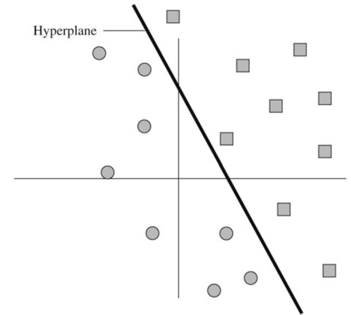
Since $\bm{\mu} \geq \bm{0}$ and $\bm{g}(\bm{x}^\ast) \geq \bm{0}$, the second of Equation 16 is equivalent to the statement that a component of $\bm{\mu}$ may be nonzero only if the corresponding constraint is active. This is a complementary slackness condition studied in LP, which states that $\bm{g}(\bm{x}^\ast)_j > 0$ implies $\mu_j = 0$ and $\mu_j > 0$ implies $\bm{g}(\bm{x}^\ast)_j = 0$.

Since $\bm{x}^\ast$ is a relative minimum point over the constraint set, it is also a relative minimum over the subset of that set defined by setting the active constraints to zero. Thus, for the resulting equality constrained problem, defined in a nbhd. of $\bm{x}^\ast$, there are Lagrange multipliers. Therefore, we conclude that first of Equation 16 holds with $\mu_j = 0$ if $g_j(\bm{x}^\ast) \neq 0$.

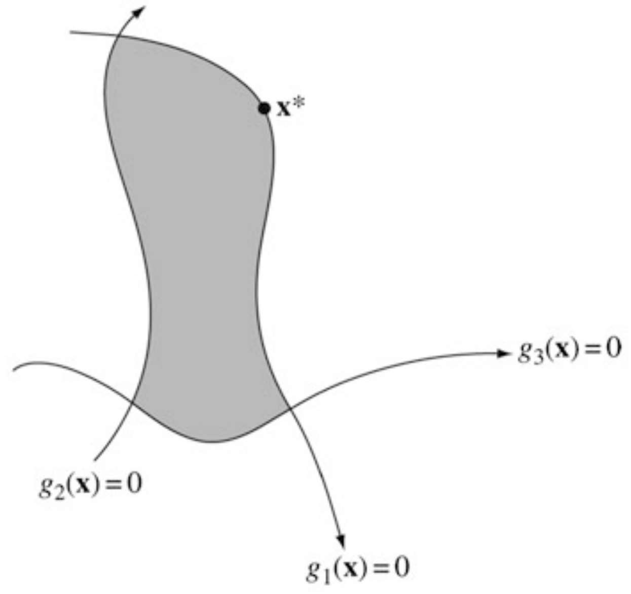
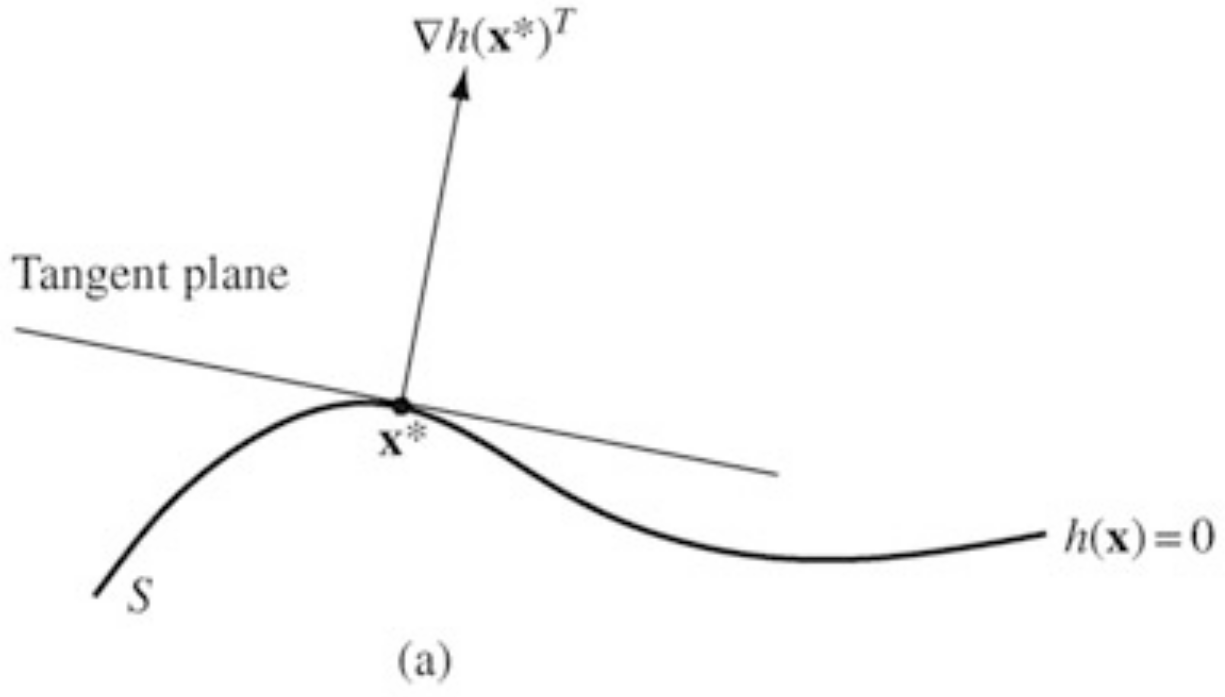
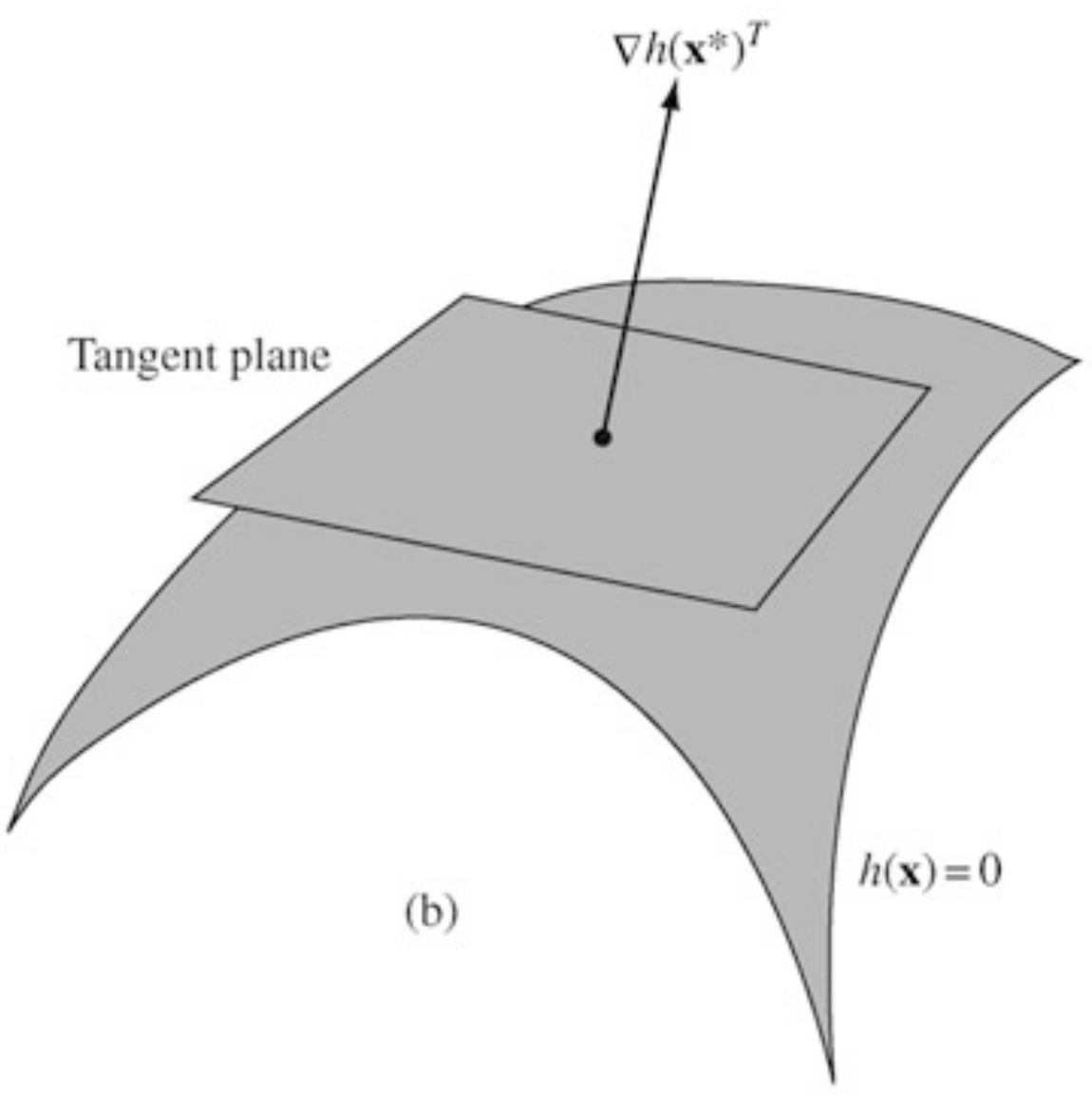
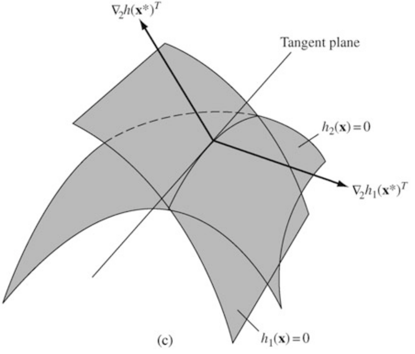
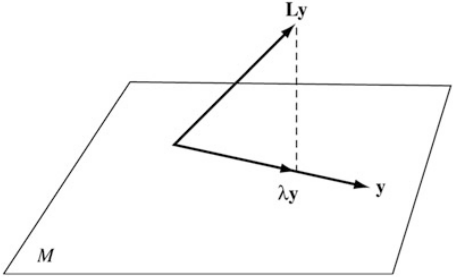
It remains to be shown that $\bm{\mu} \geq \bm{0}$. Suppose $\mu_k < 0$ for some $k \in J$. Let $S'$ and $M'$ be the surface and the tangent plane, resp., defined by all other active constraints at $\bm{x}^\ast$. By the regularity assumption, there is a $\bm{d}$ such that $\bm{d} \in M'$, that is, $\nabla \bm{h}(\bm{x}^\ast)\bm{d} = \bm{0}$ and $\nabla g_j(\bm{x}^\ast) \bm{d} = 0$ for all $j \in J$ but $j \neq k$, and $\nabla g_k(\bm{x}^\ast) \bm{d} > 0$. Multiplying this $\bm{d}$ from the right to the first of Equation 16, we have

$$\nabla f(\bm{x}^\ast) \bm{d} - \mu_k \nabla g_k(\bm{x}^\ast) \bm{d} = 0 \quad \text{or} \quad \nabla f(\bm{x}^\ast) \bm{d} = \mu_k \nabla g_k(\bm{x}^\ast) \bm{d} < 0,$$

which implies that $\bm{d}$ is a descent direction for the objective function.

Let $\bm{x}(t) \in S'$ with $\bm{x}(0) = \bm{x}^\ast$ and $\dot{\bm{x}}(0) = \bm{d}$. Then for small $t \geq 0$, $\bm{x}(t)$ is feasible – it remains on the surface of $S'$ and $g_k(\bm{x}(t)) > 0$ because $\nabla g_k(\bm{x}^\ast)\bm{d} > 0$ (that is, constrant $g_k$ becomes inactive). But

$$\frac{df}{dt}(\bm{x}(t))\Bigg\rvert_{t=0} = \nabla f(\bm{x}^\ast)\bm{d} < \bm{0}$$

which contradicts the minimality of $\bm{x}(0) = \bm{x}^\ast$.

The Lagrangian and First-Order Conditions

Introduce the Lagrangian associated with the problem, defined as

$$\mathcal L(\bm{x}, \bm{\lambda}, \bm{\mu}) = f(\bm{x}) - \bm{\lambda}^\top \bm{h}(\bm{x}) - \bm{\mu}^\top \bm{g}(\bm{x}). \qquad(17)$$

• The Lagrangian can again be viewed as an unconstrained objective function combined with the original objective with two penalized terms on constraint violations.
  • $\lambda_i$ is the penalty weight on the equality $h_i(\bm{x}) = 0$
  • $\mu_j$ is the penalty weight on the inequality $g_j(\bm{x})$.
    • There should be no penalty if $g_j(\bm{x}) > 0$, so that $\mu_j = 0$,
    • Otherwise, $\mu_j$ needs to be increased to a positive value in the Lagrangian to pump up the value of $g_j(\bm{x})$ when the Lagrangian is minimized.

First-Order Necessary Conditions

• (OVC) The original variable constraints of the problem Equation 14.
• (MSC) The multiplier sign constraints: $\bm{\lambda}$ “free” and $\bm{\mu} \geq \bm{0}$. In general, the sign of the multiplier is determined by the sense of the original constraint: (i) if it is $=$ then the sign is “free”, (ii) if it is $\leq$ or $\geq$ then the sign is $\leq$ or $\geq$, resp.
• (LDC) The Lagrangian derivative condition: the first of Equation 16
• (CSC) The complementarity slackness condition: the second of Equation 16

Example

$$\begin{align} \operatorname{minimize} & (x_1 - 1)^2 + (x_2 - 1)^2 \\ \text{subject to} & 1 - x_1^2 - x_2^2 \geq 0. \end{align}$$

The Lagrangian and the (LDC) conditions are $$\begin{align} \mathcal L(x_1, x_2, \mu(\geq 0)) &= (x_1 - 1)^2 + (x_2 - 1)^2 \\ & \phantom{123} - \mu(1 - x_1^2 - x_2^2), \\ (\text{LDC}) \;\; \nabla_\bm{x}\mathcal L(x_1, x_2, \mu) &= \begin{pmatrix} 2x_1 (1+\mu) - 2 \\ 2x_2(1+\mu) - 2 \end{pmatrix} = \bm{0}, \end{align}$$

and the (CSC) condition is $\mu(1 - x_1^2 - x_2^2) = 0$.

• From the two equations of (LDC) and $\mu \geq 0$, we conclude $x_1 = x_2$.
• We first try $\mu = 0$, which, from the two eqns. of (LDC) leads to $x_1 = x_2 = 1$ and violates the inequality constraint.
• Thus the constraint must be active, which gives rise to two possible solutions $$( x_1 = x_2 = \frac{1}{\sqrt{2}} ) \;\; \text{and} \;\; (x_1 = x_2 = \frac{-1}{\sqrt{2}}).$$
• The former, again from (LDC), makes $\mu = \sqrt{2} - 1$; while the latter makes $\mu = -\sqrt{2} - 1$, which violates (MSC).
• Thus, the only qualified first-order solution is $x_1 = x_2 = \frac{1}{\sqrt{2}}$, with the corresponding $\mu = \sqrt{2} - 1$.

Convex Problems

If $f$ is convex and $\bm{h}(\bm{x})$ is affine $\bm{Ax} - \bm{b}$, and $\bm{g}(\bm{x})$ are concave functions, then $\mathcal L(\cdot)$ is convex in $\bm{x}$ for every fixed $\bm{\lambda}$ and $\bm{\mu} (\geq \bm{0})$.

Therefore if $\bm{x}^\ast$ meets the first of Equation 16, then $\bm{x}^\ast$ is the global minimizer of the unconstrained $\mathcal L(\bm{x}, \bm{\lambda}, \bm{\mu})$ with the same $\bm{\lambda}$ and $\bm{\mu}$.

Theorem

The FONC are sufficient if $f$ is convex, $\bm{h}$ is affine, and $g_j(\bm{x})$ is concave for all $j$.

Proof

Let $\bm{x}$ be any feasible solution and $\bm{x}^\ast$, together with $\bm{\lambda}^\ast$ and $\bm{\mu}^\ast$ satisfy the FONC. Then we have

$$\begin{align} 0 &\leq \mathcal L(\bm{x}, \bm{\lambda}^\ast, \bm{\mu}^\ast) - \mathcal L(\bm{x}^\ast, \bm{\lambda}^\ast, \bm{\mu}^\ast) = f(\bm{x}) - f(\bm{x}^\ast) - (\bm{\lambda}^\ast)^\top (\bm{h}(\bm{x}) - \bm{h}(\bm{x}^\ast)) - (\bm{\mu}^\ast)^\top (\bm{g}(\bm{x}) - \bm{g}(\bm{x}^\ast)) \\ &= f(\bm{x}) - f(\bm{x}^\ast) - (\bm{\mu}^\ast)^\top (\bm{g}(\bm{x}) - \bm{g}(\bm{x}^\ast)) = f(\bm{x}) - f(\bm{x}^\ast) - \sum_{j \in J} \mu_j (g_j(\bm{x}) - g_j(\bm{x}^\ast)) \\ &= f(\bm{x}) - f(\bm{x}^\ast) - \sum_{j \in J} \mu_j g_j(\bm{x}) \leq f(\bm{x}) - f(\bm{x}^\ast). \end{align}$$

which completes the proof.

Second-Order Conditions

SONC

Suppose $\bm{x}^\ast$ is a regular point of the constraints. If $\bm{x}^\ast$ is a relative minimum point for the problem Equation 15, then there is a $\bm{\lambda} \in \mathbb{R}^m$, $\bm{\mu} \in \mathbb{R}^p$, $\bm{\mu} \geq 0$ such that Equation 16 hold and such that $$\bm{L}(\bm{x}^\ast) = \bm{F}(\bm{x}^\ast) - \bm{\lambda}^\top \bm{H}(\bm{x}^\ast) - \bm{\mu}^\top \bm{G}(\bm{x}^\ast) \qquad(18)$$ is positive semidefinite on the tangent subspace of the active constraints in $\bm{x}^\ast$.

SOSC

Sufficient conditions that a point satisfying Equation 14 be a strict relative point of the problem Equation 15 is that there exist $\bm{\lambda} \in \mathbb{R}^m$, $\bm{\mu} \in \mathbb{R}^p$ such that

$$\begin{align} \bm{\mu} &\geq 0 \\ \bm{\mu}^\top \bm{g}(\bm{x}^\ast) &= 0 \\ \nabla f(\bm{x}^\ast) - \bm{\lambda}^\top \nabla \bm{h}(\bm{x}^\ast) - \bm{\mu}^\top \nabla \bm{g}(\bm{x}^\ast) &= 0, \end{align}$$

and the Hessian matrix

$$\bm{L}(\bm{x}^\ast) = \bm{F}(\bm{x}^\ast) - \bm{\lambda}^\top \bm{H}(\bm{x}^\ast) - \bm{\mu}^\top \bm{G}(\bm{x}^\ast)$$

is positive definite on the subspace

$$M' = \left\{ \bm{d}: \nabla \bm{h}(\bm{x}^\ast)\bm{d} = 0, \nabla g_j(\bm{x}^\ast) \bm{d} = 0 \;\; \forall j \in J \right\},$$

where $J = \{j; g_j(\bm{x}^\ast) = 0, \; \mu_j > 0\}$.

Sensitivity

Sensitivity Theorem

Consider the family of problems

$$\begin{align} \operatorname{minimize} & f(\bm{x}) \\ \text{subject to} & \bm{h}(\bm{x}) = \bm{b}, \quad \bm{g}(\bm{x}) \geq \bm{c}. \end{align} \qquad(19)$$

Suppose that for $\bm{b} = \bm{0}$, $\bm{c} = \bm{0}$, there is a local solution $\bm{x}^\ast$ that is a regular point and that together with the associated Lagrange multipliers, $\bm{\lambda}, \bm{\mu} \geq \bm{0}$, satisfies the SOSC for a strict local minimum. Assume further that no active inequality constraints is degenerate.

Then for every $(\bm{b}, \bm{c}) \in \mathbb{R}^{m+p}$ in a region containing $(\bm{0}, \bm{0})$, there is a solution $\bm{x}(\bm{b}, \bm{c})$, depending continuously on $(\bm{b}, \bm{c})$, such that $\bm{x}(\bm{0}, \bm{0}) = \bm{x}^\ast$ and $\bm{x}(\bm{b}, \bm{c})$ is a relative minimum of Equation 19. Furthermore

$$\begin{align} \nabla_\bm{b} f(\bm{x}(\bm{b}, \bm{c}))\Bigg\rvert_{(\bm{0}, \bm{0})} &= \bm{\lambda}^\top, \\ \nabla_\bm{c} f(\bm{x}(\bm{b}, \bm{c}))\Bigg\rvert_{(\bm{0}, \bm{0})} &= \bm{\mu}^\top. \\ \end{align} \qquad(20)$$

Example – Soft-Margin Minimization in SVM

• In the original SVM example, the two data sets were separable, but in reality data may come in as inseparable.
• An objective function would need to be added to the model.
• Let $\bm{A}$ represent the data matrix for $\bm{a}_i$ and $\bm{B}$ represent the data for $\bm{b}_j$. Also let $\bm{1}$ denote the vector of all ones.

Optimization problem

$$\begin{align} \operatorname{minimize} & \frac{1}{2}|\bm{x}|^2 + \beta(\bm{1}^\top\bm{u} + \bm{1}^\top \bm{v}) \\ \text{subject to} & \bm{A}^\top \bm{x} + \bm{1}x_0 + \bm{u} \geq 1 \\ & -\bm{B}^\top \bm{x} - \bm{1}x_0 + \bm{v} \geq \bm{1} \\ & \bm{u} \geq \bm{0}, \; \bm{v} \geq \bm{0}. \end{align}$$

• $\{\bm{y}: \bm{x}^\top \bm{y} + x_0 = 0\}$ is the desired hyperplane.
• $u_i$ and $v_j$ represent possible error margins of $\bm{a}_i$ and $\bm{b}_j$.

Lagrangian

$$\begin{align} &\mathcal L(\bm{x},x_0, \bm{u}, \bm{v}, \bm{\xi}_A, \bm{\xi}_B) = \frac{1}{2}|\bm{x}|^2 + \beta(\bm{1}^\top \bm{u} + \bm{1}^\top \bm{v}) \\ &\phantom{234} - \bm{\xi}_A^\top (\bm{A}^\top \bm{x} + \bm{1}x_0 + \bm{u} - \bm{1}) - \bm{\xi}_B^\top (-\bm{B}^\top \bm{x} - \bm{1}x_0 + \bm{v} - \bm{1}). \end{align}$$

First-Order Conditions

• (MSC): $\phantom{231445}\bm{\xi}_A \geq \bm{0} \;\; \bm{\xi}_B \geq \bm{0}$.

• (LDC): $$\begin{align} \nabla_\bm{x}\mathcal L(\cdot) &= \bm{x} - \bm{A\xi}_A + \bm{B\xi}_B = \bm{0}, \\ \nabla_{x_0}\mathcal L(\cdot) &= -\bm{1}^\top \bm{\xi}_A + \bm{1}^\top \bm{x}_B = 0, \\ \nabla_\bm{u} \mathcal L(\cdot) &= \beta \bm{1} - \bm{\xi}_A \geq \bm{0}, \\ \nabla_\bm{v} \mathcal L(\cdot) &= \beta \bm{1} - \bm{\xi}_B \geq \bm{0}. \end{align}$$

• (CSC): $$\begin{align} \bm{\xi}_A^\top (\bm{A}^\top \bm{x} + \bm{1}x_0 + \bm{u} - \bm{1}) &= 0, \\ \bm{\xi}_B^\top (-\bm{B}^\top \bm{x} - \bm{1}x_0 + \bm{v} - \bm{1}) &= 0, \\ \bm{u}^\top(\beta \bm{1} - \bm{\xi}_A) &= 0, \\ \bm{v}^\top(\beta \bm{1} - \bm{\xi}_B) &= 0. \end{align}$$