ME/AER 647 Systems Optimization I

---

Duality Theory and Applications

Instructor: Hasan A. Poonawala

Mechanical and Aerospace Engineering
University of Kentucky, Lexington, KY, USA

Topics:
Dual function and problem
Examples
Local Duality
Sensitivity

Lagrangian and Dual Functions

The Lagrangian

Primal Optimization problem:

$$\begin{align} \min_{\bm{x}} & f(\bm{x}) \\ \text{subject to } & \bm{h}(\bm{x}) = 0\\ & \bm{g}(\bm{x}) \geq 0 \end{align}$$

Introduce the Lagrangian associated with the problem, defined as

$$\begin{align} \mathcal L(\bm{x}, \bm{\lambda}, \bm{\mu}) = f(\bm{x}) - \bm{\lambda}^\top \bm{h}(\bm{x}) - \bm{\mu}^\top \bm{g}(\bm{x}) \end{align}$$

Let $$\begin{align} \bm{h}(\bm{x})&=0 && \bm{g}(\bm{x})&\geq0, && \bm{\mu}&\geq 0,\end{align}$$ then

$$\mathcal L(\bm{x}, \bm{\lambda}, \bm{\mu}) \leq f(\bm{x})$$

The Lagrangian

$$\mathcal L(\bm{x}, \bm{\lambda}, \bm{\mu}) \leq f(\bm{x})$$

Take the infimum of both sides

$$\inf_{\bm{x}\in \Omega} \mathcal L(\bm{x}, \bm{\lambda}, \bm{\mu}) \leq \inf_{\bm{x} \in \Omega} f(\bm{x}) = p^\star$$

Dual function

$$q(\bm{\lambda},\bm{\mu}) = inf_{\bm{x}\in \Omega} \mathcal L(\bm{x}, \bm{\lambda}, \bm{\mu})$$

Lower bound property

$$q(\bm{\lambda},\bm{\mu}) \leq p^\star$$

for any dual feasible pair $(\bm{\lambda},\bm{\mu})$

Dual feasibility

The pair $(\bm{\lambda},\bm{\mu})$ is dual feasible if $\bm{\mu} \geq 0$ and $q(\bm{\lambda},\bm{\mu}) > -\infty$

The Lagrangian

$$q(\bm{\lambda},\bm{\mu}) \leq p^\star$$

• Any dual-feasible pair will provide a lower bound on the primal optimal value $p^\star$

• The best lower bound is the largest one:

Dual optimization problem

$$\begin{align} \max_{\bm{\lambda}\geq0} q(\bm{\lambda},\bm{\mu}) \end{align}$$

Dual Optimization Problem

Dual optimization problem

$$\begin{align} \max_{\bm{\lambda}\geq0} q(\bm{\lambda},\bm{\mu}) \end{align}$$

Convexity of the dual

The dual problem is a convex optimization problem

Proof

By definition, $q(\bm{\lambda},\bm{\mu})$ is the pointwise infimum of affine functions of $\bm{\lambda},\bm{\mu}$, and is therefore concave. $\bm{\mu} \geq 0$ is an affine constraint. Hence, the dual problem is maximization of a concave function with affine constraints, which is a convex optimization problem.

Duality Gap

Let $$d^\star = \max_{\bm{\lambda},\bm{\mu}\geq 0} q(\bm{\lambda},\bm{\mu})$$

Clearly,

$$d^\star \leq p^\star \quad \text{(weak duality)}$$

For convex problems that satisfy appropriate conditions, like Slater’s conditions¹, $$d^\star = p^\star$$

Generally, the duality gap is $p^\star - d^\star$, which is non-negative

1. There is a point $\bm{x}$ for which $\bm{g}(\bm{x}) \succ 0$ and $\bm{h}(\bm{x}) =0$

Dual optimization problem: Uses

• It is always convex, and provides a lower bound for the original (non-convex) problem
  • Duality gap estimates enable stopping criteria for constrained optimization
    • The estimate is simply $f(\bm{x}) - q(\bm{\lambda},\bm{\mu})$ for primal feasible $\bm{x}$ and dual feasible $\bm{\lambda},\bm{\mu}$.
  • Tells you when a problem is infeasible: heavily applied in linear programming
• For some optimization problems, the dual problem may be easier to solve
  • Duality was originally developed in the context of linear programs

Saddle Point Interpretation

When $\bm{x}$ is feasible, the lower bound property can be rewritten as $$f(\bm{x}) = \mathrm{sup}_{\bm{\lambda},\bm{\mu} \geq 0} \mathcal L(\bm{x},\bm{\lambda},\bm{\mu} ),$$

and the supremum is achieved when $(\bm{\mu}^\star)^\top \bm{g}(\bm{x}) =0$

Therefore $$\begin{align} p^\star &= \mathrm{inf}_{\bm{x} \in \Omega} f(\bm{x}) = \mathrm{inf}_{\bm{x} \in \Omega} \mathrm{sup}_{\bm{\lambda},\bm{\mu} \geq 0} \mathcal L(\bm{x},\bm{\lambda},\bm{\mu} ), \text{ and by definition} \\ d^\star &= \mathrm{sup}_{\bm{\lambda},\bm{\mu}\geq 0} \mathrm{inf}_{\bm{x} \in \Omega} \mathcal L(\bm{x},\bm{\lambda},\bm{\mu}) \end{align}$$

By weak duality,

$$\begin{align} \mathrm{sup}_{\bm{\lambda},\bm{\mu}\geq 0} \mathrm{inf}_{\bm{x} \in \Omega} \mathcal L(\bm{x},\bm{\lambda},\bm{\mu}) \leq \mathrm{inf}_{\bm{x} \in \Omega} \mathrm{sup}_{\bm{\lambda},\bm{\mu} \geq 0} \mathcal L(\bm{x},\bm{\lambda},\bm{\mu} ) \end{align}$$

and under strong duality:

$$\begin{align} \mathrm{sup}_{\bm{\lambda},\bm{\mu}\geq 0} \mathrm{inf}_{\bm{x} \in \Omega} \mathcal L(\bm{x},\bm{\lambda},\bm{\mu}) = \mathrm{inf}_{\bm{x} \in \Omega} \mathrm{sup}_{\bm{\lambda},\bm{\mu} \geq 0} \mathcal L(\bm{x},\bm{\lambda},\bm{\mu} ) \end{align}$$

Examples

Linear Least Squares

$$\begin{align} \min_{\bm{x}} \quad & \bm{x}^T \bm{x} \\ \text{s.t.} \quad & A \bm{x} = b \end{align}$$

$$\begin{align} \mathcal L(\bm{x},\bm{\lambda}) &= \bm{x}^T \bm{x} - \bm{\lambda}^\top (A \bm{x} - b)\\ \end{align}$$

$$\begin{align} \nabla_{\bm{x}}\mathcal L(\bm{x},\bm{\lambda}) &= 2 \bm{x} - A^\top \bm{\lambda} \\ \nabla_{\bm{x}}\mathcal L(\bm{x},\bm{\lambda}) =0 &\implies \bm{x} = \frac{1}{2} A^T \bm{\lambda}\\ \implies \inf_{\bm{x}}L(\bm{x},\bm{\lambda}) &= -\bm{\lambda}^\top \frac{1}{4} A A^\top \bm{\lambda} + b^\top \bm{\lambda} \\ \implies \text{Dual:} \quad & \max_{\bm{\lambda}} -\bm{\lambda}^\top \frac{1}{4} A A^\top \bm{\lambda} + b^\top \bm{\lambda} \end{align}$$

In turn, $\bm{x}^\star = \frac{1}{2} A^\top \bm{\lambda}^\star$, where $A A^\top \bm{\lambda}^\star = 2 b$¹

$\bm{x} \in \mathbb R^n$

$\bm{\lambda} \in \mathbb R^m$

1. Assuming $b \in \mathrm{span}(A)$

Support Vector Machines

$$\begin{align} \operatorname{minimize} & \frac{1}{2}\|\bm{w}\|^2 + \gamma (\bm{1}^\top\bm{u} +\bm{1}^\top \bm{v}) \\ \bm{a}_i^\top \bm{w} + \beta &\geq 1 - u_i, \quad \forall i, \\ \bm{b}_j^\top \bm{w} + \beta &\leq -1 + v_i, \quad \forall j, \\ & \bm{u} \geq \bm{0}, \; \bm{v} \geq \bm{0}. \end{align}$$

We can simplify the problem to

$$\begin{align} \operatorname{minimize}_{\bm{w},\beta,\bm{\xi}} & \frac{1}{2}\|\bm{w}\|^2 + \gamma (\bm{1}^\top\bm{\xi}) \\ \tilde{\bm{X}} \bm{w} + \beta \bm{y}_0 &\geq \bm{1} - \bm{\xi}\\ & \bm{\xi} \geq \bm{0}. \end{align}$$

Define

$$\mathcal L(\bm{w},\beta,\bm{\xi},\bm{\mu}_{X},\bm{\mu}_{\xi}) = \frac{1}{2}\|\bm{w}\|^2 + \gamma (\bm{1}^\top\bm{\xi}) - \bm{\mu}_{X}^\top \left(\tilde{\bm{X}} \bm{w} + \beta \bm{y}_0 - \bm{1} + \bm{\xi} \right) - \bm{\mu}_{\xi}^\top \xi$$

Support Vector Machines

$$\mathcal L(\bm{w},\beta,\bm{\xi},\bm{\mu}_{X},\bm{\mu}_{\xi}) = \frac{1}{2}\|\bm{w}\|^2 + \gamma (\bm{1}^\top\bm{\xi}) - \bm{\mu}_{X}^\top \left(\tilde{\bm{X}} \bm{w} + \beta \bm{y}_0 - \bm{1} + \bm{\xi} \right) - \bm{\mu}_{\xi}^\top \xi$$

$$\begin{align} &=\frac{1}{2}\|\bm{w}\|^2- \bm{\mu}_{X}^\top \tilde{\bm{X}} \bm{w} + \beta \bm{\mu}_{X}^\top \bm{y}_0 + \left(\gamma \bm{1}^\top - \bm{\mu}_{X}^\top - \bm{\mu}_{\xi}^\top \right) \bm{\xi} +\bm{1}^\top \bm{\mu}_{X} \end{align}$$

This function is convex in $\bm{w},\beta,\bm{\xi}$ (but not in all variables), with minimum given by the FONC: $$\begin{align} \nabla_{\bm{w}} \mathcal L(\bm{w},\beta,\bm{\xi},\bm{\mu}_{X},\bm{\mu}_{\xi}): && \bm{w} - \tilde{\bm{X}}^\top \bm{\mu}_{X} &= 0\\ \nabla_{\beta} \mathcal L(\bm{w},\beta,\bm{\xi},\bm{\mu}_{X},\bm{\mu}_{\xi}): &&\bm{\mu}_{X}^\top \bm{y}_0 &= 0\\ \nabla_{\bm{\xi}} \mathcal L(\bm{w},\beta,\bm{\xi},\bm{\mu}_{X},\bm{\mu}_{\xi}): &&\gamma \bm{1} - \bm{\mu}_{X} - \bm{\mu}_{\xi} &= 0\\ \end{align}$$

Support Vector Machines

Therefore, the dual of the SVM problem is: $$\begin{align} \max_{\bm{\mu}_{X},\bm{\mu}_{\xi}} \quad & -\frac{1}{2}\bm{\mu}_{X}^\top \tilde{\bm{X}} \tilde{\bm{X}}^\top \bm{\mu}_{X} +\bm{1}^\top \bm{\mu}_{X}\\ \text{s.t. }\quad & \bm{\mu}_{X}^\top \bm{y}_0 = 0\\ &\gamma \bm{1} - \bm{\mu}_{X} - \bm{\mu}_{\xi} = 0\\ & \bm{\mu}_{\xi} \geq 0 , \bm{\mu}_{X} \geq 0 \end{align}$$

Eliminating $\bm{\mu}_{\xi}$, we get the following dual SVM problem: $$\begin{align} \max_{\bm{\mu}_{X}} \quad & -\frac{1}{2}\bm{\mu}_{X}^\top \tilde{\bm{X}} \tilde{\bm{X}}^\top \bm{\mu}_{X} +\bm{1}^\top \bm{\mu}_{X}\\ \text{s.t. }\quad & \bm{\mu}_{X}^\top \bm{y}_0 = 0\\ & 0\leq \bm{\mu}_{X} \leq \gamma \bm{1} \end{align}$$

Example – The Maximal Flow Problem

Maximal flow problem

Determine the maximal flow that can be established in such a network.

$$\begin{align} \operatorname{maximize} & f \\ \text{subject to} & \sum_{j=1}^n x_{1j} - \sum_{j=1}^n x_{j1} - f = 0, \\ & \sum_{j=1}^n x_{ij} - \sum_{j=1}^n x_{ji} = 0, \quad i \neq 1, m, \\ & \sum_{j=1}^n x_{mj} - \sum_{j=1}^n x_{jm} + f = 0, \\ & 0 \leq x_{ij} \leq k_{ij}, \quad \forall i, j, \end{align}$$

where $k_{ij} = 0$ for those no-arc pairs $(i,j)$.

• Capacitated network in which two special nodes, called the source (node 1); and the sink (node $m$) are distinguished.
• All other nodes must satisfy the conservation requirement: net flow into these nodes must be zero.
  • the source may have a net outflow,
  • the sink may have a net inflow.
• The outlow $f$ of the source will equal the inflow of the sink.

Dual Linear Programs

Symmetric Form Linear Program

Linear Program (LP)

An LP is an optimization problem in which the objective function is linear in the unknowns and the constraints consist of linear (in)equalities.

Symmetric form primal LP

$$\begin{align} \operatorname{minimize}\quad & \bm{c}^\top \bm{x} \\ \text{subject to} \quad & \bm{A}\bm{x} \geq \bm{b}\\ & \bm{x} \geq \bm{0}. \end{align}$$

• $\bm{c}, \bm{x} \in \mathbb{R}^n$ are column vectors, $\bm{A} \in \mathbb{R}^{m \times n}$ a fat matrix ($m < n$), $\bm{b} \in \mathbb{R}^m$ a column vector.
• $b_i$’s, $c_i$’s and $a_{ij}$’s are fixed real constants, and the $x_i$’s are real numbers to be determined.
• We assume that each equation has been multiplied by minus unity, if necessary, so that each $b_i \geq 0$.

Example – The Diet Problem

Determine the most economical diet that satisfies the basic minimum nutritional requirements for good health

• There are available $n$ different foods.
• There are $m$ basic nutritional ingredients.
• $x_j$: How much of $j^{\text{th}}$ food is bought.

• $c_j$: unit cost of $j^{\text{th}}$ food item.
• $b_i$: Minimum amount of $i^{\text{th}}$ nutrient needed.
• $a_{ij}$: Amount of $i^{\text{th}}$ nutrient in each unit of food $j^{\text{th}}$.
  • $\bm{x}$ food purchase provides $\bm{A} \bm{x}$ of nutrients.

We want to minimize the total cost $$\min_{\bm{x}} \bm{c}^\top \bm{x}$$

subject to the nutritional constraints $$\bm{A} \bm{x} \geq \bm{b}$$

and the nonnegative constraints $$\bm{x} \geq 0$$ on the food quantities.

Example – The Resource-Allocation Problem

• A facility is capable of manufacturing $n$ different products.
• Each product may require various amounts of $m$ different resources.
• $x_j$: How much of $j^{\text{th}}$ product is produced.

• $c_j$: Profit in dollars per $j^{\text{th}}$ unit of product.
• $b_i$: Available quantity of $i^{\text{th}}$ resource.
• $a_{ij}$: How much of $i^{\text{th}}$ resource $b_i$ is needed to produce $x_j$ units of the $j^{\text{th}}$ product.
  • $\bm{x}$ product needs $\bm{A} \bm{x}$ resources to make

We wish to manufacture products at maximum revenue

$$\begin{align} \max_{\bm{x}} & \bm{c}^\top \bm{x} \end{align}$$

subject to the resource constraints

$$\begin{align} \text{subject to} & \bm{A} \bm{x} \leq \bm{b}\\ & \bm{x} \geq 0 \end{align}$$

Primal-Dual Pairs

Symmetric Form of Duality

	Primal			Dual
$\operatorname{minimize}$	$\bm{c}^\top \bm{x}$		$\operatorname{maximize}$	$\bm{b}^\top \bm{y}$
subject to	$\bm{Ax} \geq \bm{b}$		subject to	$\bm{A}^\top \bm{y} \leq \bm{c}$
	$\bm{x} \geq \bm{0}$			$\bm{y} \geq \bm{0}$

• If $\bm{A}$ is an $m \times n$ matrix, then $\bm{x}$ is an $n$-vector, $\bm{b}$ is an $m$-vector, $\bm{c}$ is an $n$ vector, and $\bm{y}$ is an $m$-vector.

• The vector $\bm{x}$ is the variable of the primal program, and $\bm{y}$ is the variable of the dual program.

Important

The roles of the primal and the dual can be reversed!

• Interchange cost and constraint vectors,
• Change minimization to maximization.

Multiplying the objective and the constraints by minus unity, the dual has the structure of the primal.

Its corresponding dual will be equivalent to the original primal.

Primal-Dual Pairs

• The dual of any linear program can be found by converting the program to the form of the primal in the previous slide.

Primal LP (Standard Form LP)

$$\begin{align} \operatorname{minimize} & \bm{c}^\top \bm{x}, \\ \text{subject to} & \bm{Ax} = \bm{b}, \quad \bm{x} \geq \bm{0} \end{align}$$

$$\begin{align} \operatorname{minimize} & \bm{c}^\top \bm{x}, \\ \text{subject to} & \bm{Ax} \geq \bm{b}, \\ & -\bm{Ax} \geq -\bm{b}, \\ & \bm{x} \geq \bm{0} \end{align}$$

Conversion to dual (Inequality Form LP)

Partition the dual vector as $(\bm{u}, \bm{v})$, we get

$$\begin{align} \operatorname{maximize} & \bm{u}^\top\bm{b} - \bm{v}^\top\bm{b}, \\ \text{subject to} & \bm{u}^\top\bm{A} - \bm{v}^\top\bm{A} \leq \bm{c}^\top, \\ & \bm{u}, \bm{v} \geq \bm{0} \end{align}$$

Letting $\bm{y} = \bm{u} - \bm{v}$, this is simplified as

$$\begin{align} \operatorname{maximize} & \bm{y}^\top \bm{b}, \\ \text{subject to} & \bm{y}^\top\bm{A} \leq \bm{c}^\top. \end{align}$$

• This is the asymmetric form of the duality relation. In this form the dual vector $\bm{y}$ is not restricted to be nonnegative.

General Procedure for Conversion

The dual of the dual is the primal!

1. The objective coefficient vector of the primal becomes the right-hand-side vector of the dual constraints,
2. The right-hand-side vector of the primal constraints becomes the objective coefficient vector of the dual,
3. The transpose of the constraint matrix of the primal becomes the constraint matrix of the dual,
4. Every primal variable corresponds to a constraint in the dual, and its sign decides the sense of the dual constraint,
5. Every primal constraint corresponds to a variable in the dual, and its sense decides the sign of the dual variable.

Relations of the primal and dual

Either side can be primal or dual

Primal/Dual		Dual/Primal
Obj. coef. vector	|	Right-hand-side
Right-hand-side	|	Obj. coef. vector
$\bm{A}$	|	$\bm{A}^\top$
Max model	|	Min model
$x_j \geq 0$	|	$j^{\text{th}}$ constraint sense: $\geq$
$x_j \leq 0$	|	$j^{\text{th}}$ constraint sense: $\leq$
$x_j$ free	|	$j^{\text{th}}$ constraint sense: $=$
$i^{\text{th}}$ constraint sense: $\leq$	|	$y_i \geq 0$
$i^{\text{th}}$ constraint sense: $\geq$	|	$y_i \leq 0$
$i^{\text{th}}$ constraint sense: $=$	|	$y_i$ free

Weak Duality

Throughout this section, we consider the primal-dual pair

$$\begin{align} \operatorname{minimize} & \bm{c}^\top \bm{x} \\ \text{subject to} & \bm{Ax} = \bm{b}, \quad \bm{x} \geq \bm{0}. \end{align} \qquad(1)$$

$$\begin{align} \operatorname{maximize} & \bm{y}^\top \bm{b} \\ \text{subject to} & \bm{y}^\top \bm{A} \leq \bm{c}^\top. \end{align}$$

Weak Duality Lemma

If $\bm{x}$ and $\bm{y}$ are feasible for the primal-dual pair, then $\bm{y}^\top\bm{b} \leq \bm{c}^\top\bm{x}$.

Proof

We have $$\bm{y}^\top \bm{b} = \bm{y}^\top \bm{Ax} \leq \bm{c}^\top \bm{x},$$ the last inequality being valid sincd $\bm{x} \geq \bm{0}$ and $\bm{y}^\top \bm{A} \leq \bm{c}^\top$.

Corollary

If $\bm{x}_0$ and $\bm{y}_0$ are feasible for the primal-dual pair and if $\bm{c}^\top \bm{x}_0 = \bm{y}_0^\top \bm{b}$, then $\bm{x}_0$ and $\bm{y}_0$ are optimal for their respective problems.

 

Strong Duality

Duality Theorem of LP

If either of the primal-dual pair problems has a finite optimal solution, so does the other, and the corresponding values of the objective functions are equal. If either problem has an unbounded objective, the other problem has no feasible solution.

Proof

Firstly, the second statement is an immediate consequence of weak duality. If the primal is unbounded and $\bm{y}$ is feasible for the dual, we must have $\bm{y}^\top \bm{b} \leq -M$ for arbitrarily large $M$, which is clearly impossible.

Let us assume that the primal has a finite optimal solution and show that the dual has a solution with the same value (recall primal/dual are reversible). We prove that if the primal problem is feasible and its minimal value is bounded from below, then the system

$$\begin{align} &\bm{Ax} = \bm{b}, \quad \bm{x} \geq \bm{0}, \\ &\bm{A}^\top \bm{y} \leq \bm{c}, \\ &\bm{c}^\top \bm{x} - \bm{b}^\top \bm{y} \leq 0 \end{align} \qquad(2)$$

has a feasible solution pair $\bm{x}$ and $\bm{y}$. The first system in Equation 2 is the primal constraint system, the second is the dual constraint system, and the third is the reversed duality gap, which, together with weak duality, implies zero-duality gap $\bm{c}^\top \bm{x} - \bm{b}^\top \bm{y} = 0$.

Strong Duality

Proof - Continued -

We first show that the dual must be feasible, since otherwise, from Farkas’s lemma the alternative system to the second system Equation 2 must be feasible, that is, there is $\bm{x}^\prime \geq \bm{0}$ such that $(\bm{Ax^\prime} = \bm{0}, \; \bm{c}^\top\bm{x}^\prime = -1)$. Let $\bm{x}$ be any given feasible solution for the primal, then the solution $\bm{x} + \alpha \bm{x}^\prime$ must also be feasible for the primal for any scalar $\alpha > 0$. But the primal objective value at this solution is $$\bm{c}^\top(x + \alpha \bm{x}^\prime) = \bm{c}^\top \bm{x} + \alpha \bm{c}^\top \bm{x}^\prime = \bm{c}^\top \bm{x} - \alpha$$ which is unbounded from below as $\alpha \rightarrow \infty$ leading to a contradiction.

Now, both the primal and the dual are feasible but suppose their optimal values are not equal; that is, the whole system Equation 2 remains infeasible. Then its alternative system must be feasible. That is, there are $(\bm{y}^\prime, \bm{x}^\prime, \tau)$ to satisfy the constraints $$\bm{Ax^\prime} - \bm{b}\tau = \bm{0}, \quad \bm{A}^\top \bm{y}^\prime - \bm{c}\tau \leq \bm{0}, \quad \bm{b}^\top \bm{y}^\prime - \bm{c}^\top \bm{x}^\prime = 1, \quad \bm{x}^\prime \geq 0, \quad \tau \geq 0. \qquad(3)$$

Case 1: $\tau > 0$ in Equation 3, then we have $$0 \geq (-\bm{y}^\prime)^\top (\bm{Ax^\prime} - \bm{b}\tau) + (\bm{x}^\prime)^\top (\bm{A}^\top \bm{y}^\prime - \bm{c}\tau) = \tau(\bm{b}^\top\bm{y}^\prime - \bm{c}^\top \bm{x}^\prime) = \tau$$ which is a contradiction.

Case 2: $\tau = 0$ in Equation 3, then we let $\bm{x}$ be any feasible solution for the primal and $\bm{y}$ be any feasible solution for the dual. Again $\bm{x} + \alpha \bm{x}^\prime$ must also be feasible for the primal and $\bm{y} + \alpha \bm{y}^\prime$ must also be feasible for the dual, and the objective gap at this pair is $$\bm{c}^\top(\bm{x} + \alpha \bm{x}^\prime) - \bm{b}^\top(\bm{y} + \alpha \bm{y}^\prime) = \bm{c}^\top \bm{x} - \bm{b}^\top \bm{y} + \alpha(\bm{c}^\top \bm{x}^\prime - \bm{b}^\top \bm{y}^\prime) = \bm{c}^\top \bm{x} - \bm{b}^\top \bm{y} - \alpha$$ which is not bounded below by $0$ as $\alpha \rightarrow \infty$ and creates a contradition to weak duality.

Sensitivity – Examples

• $p^\star = \bm{c}^\top \bm{x}^\star = \bm{b}^\top \bm{y}^\star \implies \frac{\mathrm{d}p^\star}{\mathrm{d} \bm{b}} = \bm{y}^\star$
• Dual variable $y_i$ may equivalently be considered as a marginal price of the component of $b_i$, since if $b_i$ is changed to $b_i + \Delta b_i$, the value of the optimal solution changes by $y_i\Delta b_i$.

Diet Problem

• $y_i$ is the maximum price per unit that the dietitian would be willing to pay for a small amount of the $i^{\text{th}}$ nutrient.
• Decreasing the amount of the nutrient that must be supplied by food will reduce the food bill by $y_i$ dollars per unit.

Production Problem

• Manufacturer must select levels $x_1, x_2, \ldots, x_n$ of $n$ production activites in order to meet certain required levels of output $b_1, b_2, \ldots, b_m$ while minimizing production costs.
• $y_i$’s are the marginal prices of the outputs.
• They show directly how much the production cost varies if a small change is made in the output levels.

Theorem

The minimal value function $z(\bm{b})$ of the linear program Equation 1 is a convex function, and the optimal dual solution $\bm{y}^\ast$ is a subgradient vector of the function at $\bm{b}$, written as $\nabla z(\bm{b}) = \bm{y}^\ast$.

Sensitivity — Subgradient Theorem

Theorem

The minimal value function $z(\bm{b})$ of the linear program Equation 1 is a convex function, and the optimal dual solution $\bm{y}^\ast$ is a subgradient vector of the function at $\bm{b}$, written as $\nabla z(\bm{b}) = \bm{y}^\ast$.

Proof

Let $\bm{x}^1$ and $\bm{x}^2$ be two optimal solutions of Equation 1 corresponding to two right-hand-side vectors $\bm{b}^1$ and $\bm{b}^2$, resp. Then, for any scalar $0 \leq \alpha \leq 1$, $\alpha \bm{x}^1 + (1-\alpha)\bm{x}^2$ is a feasible solution of Equation 1 with $\bm{b} = \alpha \bm{b}^1 + (1-\alpha)\bm{b}^2$ so that the minimal value is

$$z(\alpha \bm{b}^1 + (1-\alpha)\bm{b}^2) \leq \bm{c}^\top (\alpha \bm{x}^1 + (1-\alpha)\bm{x}^2) = \alpha \bm{c}^\top \bm{x}^1 + (1-\alpha)\bm{c}^\top \bm{x}^2 = \alpha z(\bm{b}^1) + (1-\alpha)z(\bm{b}^2)$$

which implies the first claim.

Furthermore, let $\bm{y}^1$ be the optimal dual solution with $\bm{b} = \bm{b}^1$. Note that $\bm{y}^1$ remains feasible for the dual of primal with $\bm{b} = \bm{b}^2$ because the dual feasible region is independent of changes in $\bm{b}$. Thus

$$\begin{align} z(\bm{b}^2) - z(\bm{b}^1) &= \bm{c}^\top \bm{x}^2 - (\bm{y}^1) & \text{(zero-duality gap theorem)} \\ &\geq (\bm{y}^1)^\top \bm{b}^2 - (\bm{y}^1)^\top \bm{b}^1 & \text{(weak duality)} \\ &= (\bm{y}^1)^\top (\bm{b}^2 - \bm{b}^1), \end{align}$$

which proves the second claim.

Sensitivity

• The Lagrange multipliers associated with a constrained minimization problem have an interpretation as prices, similar to the prices in LP.

• Let a minimal solution $\bm{x}^\ast$ be a regular point and $\bm{\lambda}^\ast$ be the corresponding Lagrange multiplier vector. Consider the family of problems

$$\begin{align} z(\bm{b}) = &\operatorname{minimize} &f(\bm{x}) \phantom{1234} & \\ & \text{subject to} & \bm{h}(\bm{x}) = \bm{b}, & \bm{b} \in \mathbb{R}^m. \end{align} \qquad(4)$$

• For sufficiently small $|\bm{b}|$, the problem will have a solution point $\bm{x}(\bm{b})$ near $\bm{x}(\bm{0}) = \bm{x}^\ast$.
  • For each of these solutions, there is a corresponding minimum value $z(\bm{b}) = f(\bm{x}(\bm{b}))$.
  • The components of the gradient of this function can be regarded as the incremental rate of change in value per unit change in the constraint requirement.

Sensitivity

Sensitivity Theorem

Consider the family of problems Equation 4. Suppose that for every $\bm{b} \in \mathbb{R}^m$ in a region containing $\bm{0}$, its minimizer $\bm{x}(\bm{b})$ is continuously differentiable depending on $\bm{b}$. Let $\bm{x}^\ast = \bm{x}(\bm{0})$ with the corresponding Lagrange multiplier $\bm{\lambda}^\ast$. Then

$$\nabla z(\bm{0}) = \nabla_\bm{b} f(\bm{x}(\bm{b})) \Bigg\rvert_{\bm{b}=\bm{0}} = \left(\bm{\lambda}^\ast\right)^\top.$$

Sensitivity

Sensitivity Theorem

Consider the family of problems Equation 4. Suppose that for every $\bm{b} \in \mathbb{R}^m$ in a region containing $\bm{0}$, its minimizer $\bm{x}(\bm{b})$ is continuously differentiable depending on $\bm{b}$. Let $\bm{x}^\ast = \bm{x}(\bm{0})$ with the corresponding Lagrange multiplier $\bm{\lambda}^\ast$. Then

$$\nabla z(\bm{0}) = \nabla_\bm{b} f(\bm{x}(\bm{b})) \Bigg\rvert_{\bm{b}=\bm{0}} = \left(\bm{\lambda}^\ast\right)^\top.$$

Proof

Using the chain rule and taking derivatives with respect to $\bm{b}$ on both sides of

$$\bm{b} = \bm{h}(\bm{x}(\bm{b}))$$

at $\bm{b} = \bm{0}$, we have

$$\bm{I} = \nabla_\bm{b} \bm{h}(\bm{x}(\bm{b})) \Bigg\rvert_{\bm{b}=\bm{0}} = \nabla_\bm{x} \bm{h}(\bm{x}(\bm{0}))\nabla_\bm{b}\bm{x}(\bm{0}) = \nabla_\bm{x}\bm{h}(\bm{x}^\ast)\nabla_\bm{b}\bm{x}(\bm{0}).$$

On the other hand, using the chain rule and the first-order condition for $\bm{x}^\ast$ and the above matrix equality

$$\nabla_\bm{b} f(\bm{x}(\bm{b})) \Bigg\rvert_{\bm{b}=\bm{0}} = \nabla f(\bm{x}(\bm{0})) \nabla_{\bm{b}}\bm{x}(\bm{0}) = \nabla f(\bm{x}^\ast) \nabla_{\bm{b}}\bm{x}(\bm{0}) = \left(\bm{\lambda}^\ast\right)^\top \nabla_\bm{x} \bm{h}(\bm{x}^\ast) \nabla_\bm{b} \bm{x}(\bm{0}) = \left(\bm{\lambda}^\ast\right)^\top.$$

Local Duality and the Lagrangian Method

Local Duality

To solve the dual optimization problem, we need to solve

$$\begin{align} \max_{\bm{\lambda}\geq0} q(\bm{\lambda},\bm{\mu}) \end{align}$$

The dual function $q(\bm{\lambda},\bm{\mu})$ is defined using a constrained optimization problem:

$$q(\bm{\lambda},\bm{\mu}) = inf_{\bm{x}\in \Omega} \mathcal L(\bm{x}, \bm{\lambda}, \bm{\mu})$$

 

Can we replace the inner constrained optimization with unconstrained local optimization?:

$$\begin{align} \operatorname{Modified\ Dual\ Opt:\quad}\max_{\bm{\lambda}\geq0} \phi(\bm{\lambda},\bm{\mu}) \end{align}$$ where

$$\phi(\bm{\lambda},\bm{\mu}) = inf_{\bm{x} \in \mathcal N(\bm{x}^\star)} \mathcal L(\bm{x}, \bm{\lambda}, \bm{\mu})$$

Local duality answers ‘yes’ in some cases.

Example

$$\begin{align} \operatorname{minimize} & -xy \\ \text{subject to} & (x-3)^2 + y^2 = 5. \end{align}$$

Dual Function

$$q(\lambda) = -x^\star y^{\star} = -8 \operatorname{\quad(a\ constant)}$$

First-Order Necessary Conditions

$$\begin{align} -y - (2x - 6)\lambda &= 0 \\ -x - 2y\lambda &= 0. \end{align}$$ together with the constraint. These equations have a solution at $$x^\star = 4, \quad y^{\star} = 2, \quad \lambda^{\star} = -1.$$ The Hessian of the corresponding Lagrangian is $$\bm{L} = \begin{bmatrix} 2 & -1 \\ -1 & 2 \end{bmatrix}.$$ Since this is positive definite, we conclude that the solution obtained is a local minimum (it is, in fact, a global minimum).

Local Duality

Since $\bm{L}$ is positive definite, we can apply the local duality theory near this solution. $$\phi(\lambda) = \operatorname{min}_{x,y} \left\{-xy - \lambda \left[(x-3)^2 + y^2 - 5\right]\right\},$$ which leads to $$\phi(\lambda) = \frac{-4\lambda - 4\lambda^3 + 80\lambda^5}{(4\lambda^2 - 1)^2}$$ valid for $\lambda < -\frac{1}{2}$. It can be verified that $\phi$ has a local maximum at $\lambda = -1$. Plugging this value back in Equation 8 and maximizing (unconstrained) over $x$ and $y$ yields the same maximizers as before.

Local Duality

Nonlinear Programming Problem

$$\begin{align} \operatorname{minimize} & f(\bm{x}), & f, \bm{h} \in C^2, \\ \text{subject to} & \bm{h}(\bm{x}) = \bm{0}, & \bm{x} \in \mathbb{R}^n, \bm{h}(\bm{x}) \in \mathbb{R}^m. \end{align} \qquad(5)$$

Everything we do can be easily extended to problems having inequality as well as equality constraints for the price of a somewhat more involved notation.

• Assume that $\bm{x}^\ast$ is a regular point of the constraints.
  • There is then a Lagrange multiplier vector $\bm{\lambda}^\ast$ such that

$$\nabla f(\bm{x}^\ast) - \left(\bm{\lambda}^\ast\right)^\top \nabla \bm{h} (\bm{x}^\ast) = \bm{0}, \qquad(6)$$

and the Hessian of the Lagrangian $\ell(\bm{x}, \bm{\lambda}^\ast) = f(\bm{x}) - \left(\bm{\lambda}^\ast\right)^\top \bm{h}(\bm{x})$

$$\bm{L}(\bm{x}^\ast) = \bm{F}(\bm{x}^\ast) - \left(\bm{\lambda}^\ast\right)^\top \bm{H}(\bm{x}^\ast) \qquad(7)$$

must be positive semidefinite on the tangent subspace

$$M = \{\bm{x}: \nabla \bm{h}(\bm{x}^\ast) = \bm{0}\}.$$

Local Convexity Assumption

We assume that the Hessian $\bm{L(\bm{x}^\ast)}$ is positive definite. (We mean that $\bm{L(\bm{x}^\ast)}$ on the whole space $\mathbb{R}^n$, not just on the subspace $M$.)

This assumption guarantees that the Lagrangian $\ell(\bm{x}, \bm{\lambda}^\ast)$ is locally convex at $\bm{x}^\ast$.

• With this assumption, the point $\bm{x}^\ast$ is not only a local solution to the constrained problem Equation 5; it is also a local solution to the unconstrained problem

$$\begin{align} \operatorname{minimize} & \ell(\bm{x}, \bm{\lambda}^\ast) = f(\bm{x}) - \left( \bm{\lambda}^\ast \right)^\top \bm{h}(\bm{x}) \end{align} \qquad(8)$$

• For any $\bm{\lambda}$ sufficiently close to $\bm{\lambda}^\ast$, the function $\ell(\bm{x}, \bm{\lambda})$ will have a local minimum point at a point $\bm{x}$ near $\bm{x}^\ast$.
  • This follows by noting that by the implicit function theorem, the equation $$\nabla f(\bm{x}) - \bm{\lambda}^\top \nabla \bm{h} (\bm{x}) = \bm{0}$$

has a solution $\bm{x}$ near $\bm{x}^\ast$ when $\bm{\lambda}$ is near $\bm{\lambda}^\ast$ because $\bm{L}^\ast$ is positive definite.

Local Duality

• Thus, locally there is a unique correspondence between $\bm{\lambda}$ and $\bm{x}$ through the solution of the unconstrained problem Equation 8. $$\begin{align} \operatorname{minimize} & \ell(\bm{x}, \bm{\lambda}) = f(\bm{x}) - \bm{\lambda}^\top \bm{h}(\bm{x}). \end{align} \qquad(9)$$

  • This correspondence is continuously differentiable.

• Near $\bm{\lambda}^\ast$ we define the dual function $\phi$ by the equation $$\phi(\bm{\lambda}) \triangleq \operatorname{min}_{\bm{x} \in \mathcal{N}(\bm{x}^\ast)} \left[ \ell(\bm{x}, \bm{\lambda}) = f(\bm{x}) - \bm{\lambda}^\top \bm{h}(\bm{x}) \right] \qquad(10)$$

• We are then able to show that locally the original constrained problem Equation 8 is equivalent to unconstrained local maximization of the dual function $\phi$ with respect to $\bm{\lambda}$.

  • Denote by $\bm{x}(\bm{\lambda})$ the unique solution to Equation 9 in the neighborhood of $\bm{x}^\ast$.

Lemma 1

The dual function $\phi$ has gradient $$\nabla \phi(\bm{\lambda}) = -\bm{h}(\bm{x}(\bm{\lambda}))^\top. \qquad(11)$$

Proof

We have explicitly from Equation 10 $$\phi(\bm{\lambda}) = f(\bm{x}(\bm{\lambda})) - \bm{\lambda}^\top \bm{h}(\bm{x}(\bm{\lambda})).$$ Thus $$\nabla \phi(\bm{\lambda}) = \left[ \nabla f(\bm{x}(\bm{\lambda})) - \bm{\lambda}^\top \nabla \bm{h}(\bm{x}(\bm{\lambda})) \right] \nabla \bm{x}(\bm{\lambda}) - \bm{h}(\bm{x}(\bm{\lambda}))^\top.$$ Since the first term on the right vanishes by the defition of $\bm{x}(\bm{\lambda})$ (the unique solution to Equation 9), we obtain Equation 11.

Lemma 2

The Hessian of the dual function is $$\bm{\Phi}(\bm{\lambda}) = -\nabla \bm{h}(\bm{x}(\bm{\lambda}))\bm{L}^{-1}(\bm{x}(\bm{\lambda}), \bm{\lambda}) \nabla \bm{h}(\bm{x}(\bm{\lambda}))^\top. \qquad(12)$$

Proof

By Lemma 1, $\bm{\Phi}(\bm{\lambda}) = -\nabla \bm{h}(\bm{x}(\bm{\lambda})) \nabla \bm{x}(\bm{\lambda})$.

Differentiating $\nabla f(\bm{x}(\bm{\lambda})) - \bm{\lambda}^\top \nabla \bm{h}(\bm{x}(\bm{\lambda})) = \bm{0}$ with respect to $\bm{\lambda}$, we obtain

$$\bm{L}(\bm{x}(\bm{\lambda}), \bm{\lambda})\nabla \bm{x}(\bm{\lambda}) - \nabla \bm{h}(\bm{x}(\bm{\lambda}))^\top = \bm{0}.$$

Solving for $\nabla \bm{x}(\bm{\lambda})$ and substituting back to the first equation, we are through.

Local Duality Theorem

Local Duality Theorem

Suppose that the problem $$\begin{align} \operatorname{minimize} & f(\bm{x}) \\ \text{subject to} & \bm{h}(\bm{x}) = \bm{0} \end{align}$$ has a local solution at $\bm{x}^\ast$ with corresponding value $r^\ast$ and Lagrange multiplier $\bm{\lambda}^\ast$. Suppose also that $\bm{x}^\ast$ is a regular point of the constraints and that the corresponding Hessian of the Lagrangian $\bm{L}^\ast = \bm{L}(\bm{x}^\ast)$ is positive definite. Then the dual problem $$\begin{align} \operatorname{maximize} & \phi(\bm{\lambda}) \end{align}$$ has a local solution at $\bm{\lambda}^\ast$ with corresponding value $r^\ast$ and $\bm{x}^\ast$ as the point corresponding to $\bm{\lambda}^\ast$ in the definition of $\phi$.

Proof

It is clear that $\bm{x}^\ast$ corresponds to $\bm{\lambda}^\ast$ in the definition of $\phi$. Now at $\bm{\lambda}^\ast$ we have by Lemma 1, $$\nabla \phi(\bm{\lambda}^\ast) = -\bm{h}(\bm{x}^\ast)^\top = \bm{0},$$ and by Lemma 2, the Hessian of $\phi$ is negative definite. Thus $\bm{\lambda}^\ast$ satisfies the SOSC for an unconstrained maximum point of $\phi$. The corresponding value $\phi(\bm{\lambda}^\ast)$ is found from the definition of $\phi$ to be $r^\ast$.

Inequality Constraints

$$\begin{align} \operatorname{minimize} & f(\bm{x}), & f \in C^2, \;\; \bm{x}\in \mathbb{R}^n \\ \text{subject to} & \bm{h}(\bm{x}) = \bm{0}, & \bm{h} \in \mathbb{C}^2, \;\; \bm{h}(\bm{x}) \in \mathbb{R}^m, \\\ & \bm{g}(\bm{x}) \geq \bm{0}, & \bm{g} \in C^2, \;\; \bm{g}(\bm{x}) \in \mathbb{R}^p. \end{align} \qquad(13)$$

• Suppose $\bm{x}^\ast$ is a local solution of Equation 13 and is a regular point of the constraints.
  • Then, there are Lagrange multipliers $\bm{\lambda}^\ast$ and $\bm{\mu}^\ast \geq \bm{0}$ such that $$\begin{align} \nabla f(\bm{x}^\ast) - \left(\bm{\lambda}^\ast \right)^\top \nabla \bm{h}(\bm{x}^\ast) - \left(\bm{\mu}^\ast\right)^\top \nabla \bm{g}(\bm{x}^\ast) &= \bm{0}, \\ \left(\bm{\mu}^\ast\right)^\top \bm{g}(\bm{x}^\ast) = 0. \end{align}$$
• Local convexity assumption: Hessian of the Lagrangian is positive definite on the whole space. $$\bm{L}(\bm{x}^\ast) = \bm{F}(\bm{x}^\ast) - \left(\bm{\lambda}^\ast\right)^\top \bm{H}(\bm{x}^\ast) - \left(\bm{\mu}^\ast\right)\bm{G}(\bm{x}^\ast) \succ \bm{0}.$$
• For $\bm{\lambda}$ and $\bm{\mu} \geq \bm{0}$ near $\bm{\lambda}^\ast$ and $\bm{\mu}^\ast$ we can define the dual function $$\phi(\bm{\lambda}, \bm{\mu}) \triangleq \operatorname{min}_{\bm{x} \in \mathcal{N}(\bm{x}^\ast)} \left[ \ell(\bm{x}, \bm{\lambda}, \bm{\mu}) = f(\bm{x}) - \bm{\lambda}^\top \bm{h}(\bm{x}) - \bm{\mu}^\top \bm{g}(\bm{x}) \right],$$ where the minimum is taken locally near $\bm{x}^\ast$.
• Then it is easy to show, paralleling the devlopment above for equality constraints, that $\phi$ achieves a local maximum with respect to $\bm{\lambda}$, $\bm{\mu} \geq \bm{0}$ at $\bm{\lambda}^\ast$, $\bm{\mu}^\ast$.

Partial Duality

• It is not necessary to include the Lagrange multipliers of all the constraints of a problem in the definition of the dual function.
• In general, if the local convexity assumption holds, local duality can be defined with respect to any subset of function constraints.
  • For example, in problem Equation 13 we might define the dual with respect to only the equality constraints $$\phi(\bm{\lambda}) = \operatorname{min}_{\bm{g}(\bm{x}) \geq \bm{0}} \left\{f(\bm{x}) - \bm{\lambda}^\top \bm{h}(\bm{x}) \right\},$$ where the minimum is taken locally near the solution $\bm{x}^\ast$ but constrained by the remaining constraints $\bm{g}(\bm{x}) \geq \bm{0}$.
• Again, the dual function defined in this way will achieve a local maximum at the optimal Lagrange multiplier $\bm{\lambda}^\ast$.
• The partial dual is especially useful when constraints $\bm{g}(\bm{x}) \geq \bm{0}$ are simple such as $\bm{x} \geq \bm{0}$ or in a box where many efficient algorithms are available.
  • Steepest descent projection, interior ellipsoidal-trust region methods, etc.

Dual Steepest Ascent

The modified dual optimization problem is $$\begin{align} \max_{\bm{\lambda}\geq0} \phi(\bm{\lambda},\bm{\mu}) \end{align}$$ which has the same optimum as the true dual optimization problem, under appropriate conditions.

From Lemma 1, the gradient at $(\bm{\lambda},\bm{\mu})$ is given by the constraint functions evaluated at the optimum of $$\min_{\bm{x} } \mathcal L(\bm{x}, \bm{\lambda}, \bm{\mu})$$

To solve the modified dual optimization problem we run the following iterations:

1. Find the unconstrained minimizer $\bm{x}_k$ in $\bm{x}$ of the Lagrangian with current iterates $\bm{\lambda}_k,\bm{\mu}_k$
2. Use this minimizer to (easily) calculate the gradient of the modified dual function $\phi(\bm{\lambda},\bm{\mu})$ at $\bm{\lambda}_k,\bm{\mu}_k$
3. Get the next iterate $\bm{\lambda}_{k+1},\bm{\mu}_{k+1}$ by taking a step in the direction of this gradient

The Lagrangian Method: Dual Steepest Ascent

• According to Lemma 1, the gradient of $\phi$ is available almost without cost once $\phi$ is evaluated.
  • Any of the standard algorithms discussed for unconstrained optimization can be used for solving the unconstrained Lagrangian problem to evaluate the dual gradient vector.
  • The iterative scheme is simply, starting from any initial pairs $\left(\bm{x}_0, \bm{\lambda}_0, \bm{\mu}_0(\geq \bm{0})\right)$,

$$\begin{align} \bm{x}_{k+1} &:= \operatorname{arg}\,\operatorname{min}_\bm{x} \ell(\bm{x}, \bm{\lambda}_k, \bm{\mu_k}), \\ \bm{\lambda}_{k+1} &:= \bm{\lambda}_k - \frac{1}{c}\bm{h}(\bm{x}_{k+1}), \\ \bm{\mu}_{k+1} &:= \operatorname{max} \left\{\bm{0}, \, \bm{\mu}_k - \frac{1}{c}\bm{g}(\bm{x}_{k+1}) \right\}. \end{align}$$

Here, $c$ is the first-order Lipschitz constant of the dual function $\phi(\bm{\lambda}, \bm{\mu})$.

• Without some special properties, however, the method as a whole can be costly to execute.
  • Every evaluation of $\phi$ requires the solution of an unconstrained problem in the unknown $\bm{x}$.
• Convergence speed: identical to those discussed for solving unconstrained problems.
  • If the dual objective is strongly concave, the convergence rate is governed by the eigenvalue structure of the Hessian of the dual function $\phi$: $\bm{\Phi} = -\nabla \bm{h}(\bm{x}^\ast)\left(\bm{L}^\ast\right)^{-1}\nabla \bm{h}(\bm{x}^\ast)^\top$.
  • The rate of convergence is $\frac{(B-b)^2}{(B+b)^2}$, where $B$ and $b$ are the largest and smallest eigenvalues of $\bm{\Phi}$.

The Augmented Lagrangian and Interpretations

• One of the most effective general classes of NLP methods is the augmented Lagrangian methods.
• Alternatively referred to as methods of multiplier.

The Augmented Lagrangian

• These methods can be veiwed as a combination of penalty functions and local duality methods.
  • The two concepts work together to eliminate many of the disadvantages associated with either method alone.
• The augmented Lagrangian for the equality constrained problem is the function $$\ell_c(\bm{x}, \bm{\lambda}) = f(\bm{x}) - \bm{\lambda}^\top \bm{h}(\bm{x}) + \frac{c}{2}\left|\bm{h}(\bm{x})\right|^2$$ for some positive constant $c$.
• From a penalty function viewpoint, the augmented Lagrangian, for a fixed value of the vector $\bm{\lambda}$ is simply the Lagrange penalty function for the problem $$\begin{align} \operatorname{minimize} & f(\bm{x}) + \frac{1}{2}c\left|\bm{h}(\bm{x})\right|^2, \\ \text{subject to} & \bm{h}(\bm{x}) = \bm{0}, \quad \bm{x} \in \Omega \end{align}$$
• This problem is clearly equivalent to the original equality constrained problem since the combinations of the constraints adjoined to $f(\bm{x})$ do not affect the minimum point or the minimum value.
• A typical step of an augmented Lagrangian method starts with a vector $\bm{\lambda}_k$. Then $\bm{x}(\bm{\lambda}_k)$ is found as the minimum point of $$\bm{x}(\bm{\lambda}_k) = \operatorname{arg} \operatorname{min} f(\bm{x}) - \bm{\lambda}_k^\top \bm{h}(\bm{x}) + \frac{1}{2}c\left|\bm{h}(\bm{x})\right|^2, \quad \text{subject to} \quad \bm{x} \in \Omega.$$
• Next, $\bm{\lambda}_k$ is updated to $\bm{\lambda}_{k+1}$: $$\bm{\lambda}_{k+1} = \bm{\lambda}_k - c\bm{h}(\bm{x}(\bm{\lambda}_k)).$$

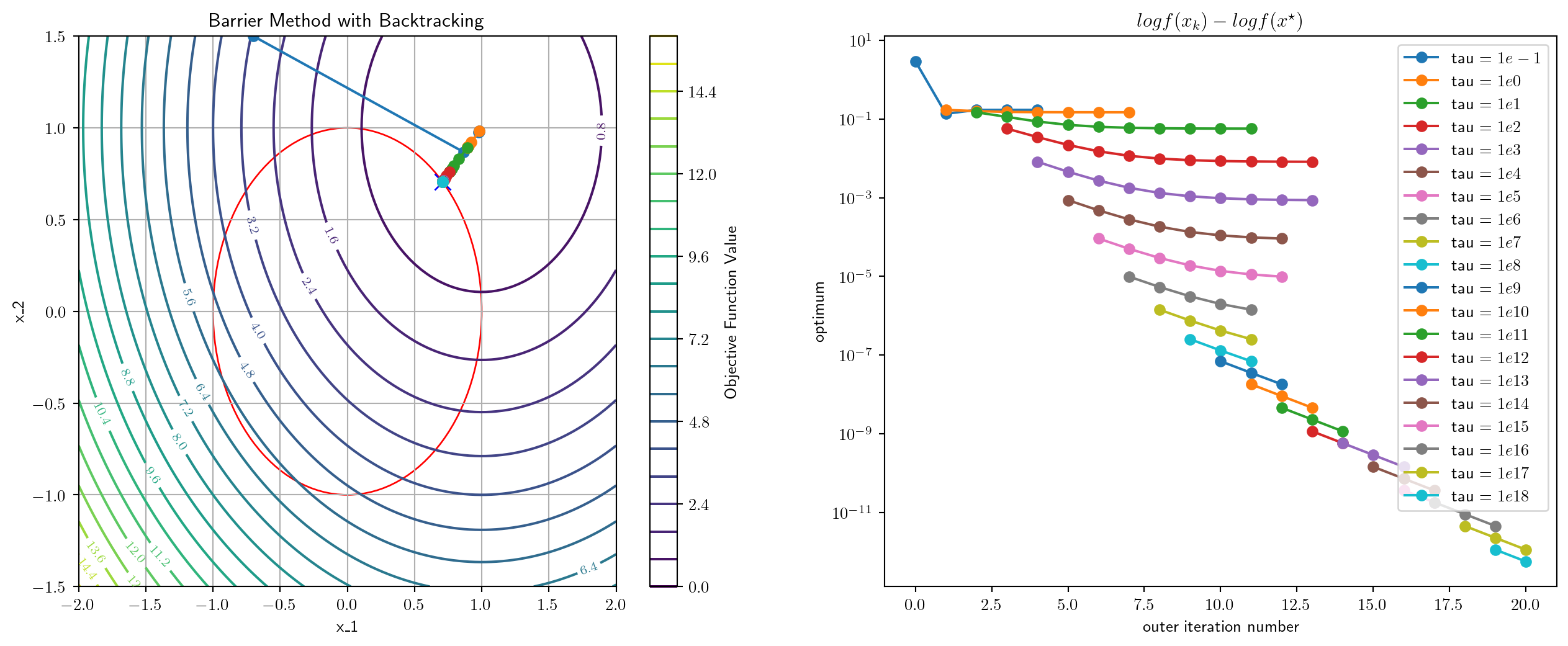
Example

0.5199909210205078 msec elapsed for NM
[0.70710678 0.70710678]

The Augmented Lagrangian

• Whereas the original Lagrangian may not be convex near the solution, and hence the standard duality method cannot be applied, the term $\frac{1}{2}c\left|\bm{h}(\bm{x})\right|^2$ tends to “convexify” the Lagrangian.
  • For sufficiently large $c$, the Lagrangian will indeed be locally convex.
  • Thus, the duality method can be employed, and the corresponding dual problem can be solved by an iterative process in $\bm{\lambda}$.
  • This viewpoint leads to the development of additional multiplier adjustment processes.
• The main iteration in augmented Lagrangian methods is with respect to $\bm{\lambda}$.
  • The penalty parameter $c$ may also be adjusted during the process!
  • As in ordinary penalty function methods, the sequence of $c$’s is usually preselected;
    • $c$ is either held fixed,
    • is increased toward a finite value,
    • or tends (slowly) toward infinity.
  • In this method, it is not necessary for $c$ to go to infinity.
    • In fact, it may remain of relatively modest value.
    • The ill-conditioning usually associated with the penalty function approach is mediated.

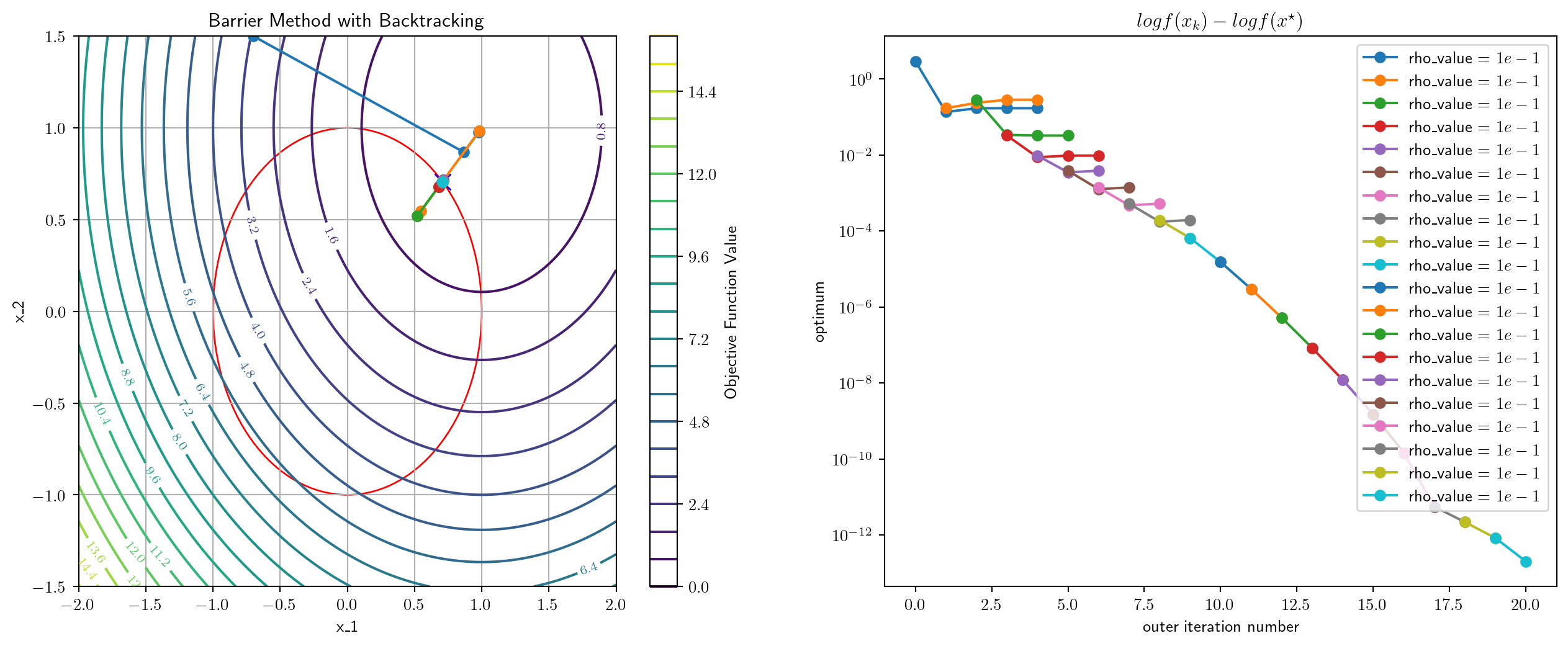
Example: Penalty Method

0.9369850158691406 msec elapsed for NM
[0.70710678 0.70710678]

The Penalty Viewpoint

Lemma

Let $\bm{A}$ and $\bm{B}$ be $n$-by-$n$ symmetric matrices. Suppose that $\bm{B}$ is positive semidefinite and $\bm{A}$ is positive definite on the subspace $\bm{Bx} = \bm{0}$. Then there is a $c^\ast$ such that for all $c \geq c^\ast$ the matrix $\bm{A} + c\bm{B}$ is positive definite.

Proof

Suppose to the contrary that for every $k$ there were an $\bm{x}_k$ with $|\bm{x}_k| = 1$ such that $\bm{x}_k^\top (\bm{A} + k\bm{B})\bm{x}_k \leq 0$. The sequence $\left\{\bm{x}_k\right\}$ must have a convergent subsequence converging to a limit $\bar{\bm{x}}$. Now since $\bm{x}_k^\top \bm{B} \bm{x}_k \geq 0$, it follows that $\bar{\bm{x}}^\top \bm{B} \bar{\bm{x}} = 0$. It also follows that $\bar{\bm{x}}^\top \bm{A} \bar{\bm{x}} \leq 0$. However, this contradicts the hypothesis of the lemma.

• This lemma applies to the Hessian of the augmented Lagrangian, evaluated at the optimal solution pair $\bm{x}^\ast$, $\bm{\lambda}^\ast$. $$\begin{align} \bm{L}_c(\bm{x}^\ast, \bm{\lambda}^\ast) = \bm{F}(\bm{x}^\ast) - \left(\bm{\lambda}^\ast\right)^\top\bm{H}(\bm{x}^\ast) + c\nabla \bm{h}(\bm{x}^\ast)^\top \bm{h}(\bm{x}^\ast) = \bm{L}(\bm{x}^\ast) + c\nabla \bm{h}(\bm{x}^\ast)^\top \nabla \bm{h}(\bm{x}^\ast). \end{align}$$

  • The first term, the Hessian of the normal Lagrangian, is positive definite on the subspace $\nabla \bm{h}(\bm{x}^\ast) = \bm{0}$. This corresponds to the matrix $\bm{A}$ in the lemma.
  • The matrix $\nabla \bm{h}(\bm{x}^\ast)^\top \nabla \bm{h}(\bm{x}^\ast)$ is positive semidefinite and corresponds to $\bm{B}$ in the lemma.
    • It follows that there is a $c^\ast$ such that for all $c > c^\ast$, $\bm{L}_c(\bm{x}^\ast, \bm{\lambda}^\ast)$ is positive definite.

• This leads directly to the first basic result concerning augmented Lagrangian.

The Penalty Viewpoint

Proposition

Assume that the second-order sufficiency conditions for a local minimum are satisfied at $\bm{x}^\ast$, $\bm{\lambda}^\ast$. Then there is a $c^\ast$ such that for all $c \geq c^\ast$, the augmented Lagrangian $\ell_c(\bm{x}, \bm{\lambda}^\ast)$ has a local minimum point at $\bm{x}^\ast$.

• By continuity, for any $\bm{\lambda}$ near $\bm{\lambda}^\ast$, the augmented Lagrangian has a unique local minimum point near $\bm{x}^\ast$.
• This correspondence defines a continuous function.
  • If a value of $\bm{\lambda}$ can be found such that $\bm{h}(\bm{x}(\bm{\lambda})) = \bm{0}$, then that $\bm{\lambda}$ must in fact be $\bm{\lambda}^\ast$.
    • This is because $\bm{x}(\bm{\lambda})$ satisfies the necessary conditions of the original problem.
• Therefore, the problem of determining the proper value of $\bm{\lambda}$ can be viewed as one of solving the equation $$\bm{h}(\bm{x}(\bm{\lambda})) = \bm{0}.$$
• For this purpose the iterative process $$\bm{\lambda}_{k+1} = \bm{\lambda}_k - c \bm{h}(\bm{x}(\bm{\lambda}_k)),$$ is a method of successive approximation (such as fixed-point iteration).
  • This process will converge linearly in a neighborhood around $\bm{\lambda}^\ast$ although a rigorous proof is somewhat complex.

Example

$$\begin{align} \operatorname{minimize} & 2x^2 + 2xy + y^2 - 2y, \\ \text{subject to} & x = 0. \end{align}$$

• The augmented Lagrangian for this problem is

$$\ell_c(x, y, \lambda) = 2x^2 + 2xy + y^2 - 2y - \lambda x + \frac{1}{2}cx^2.$$

• The minimum can be found analytically to be

$$x = \frac{-(2-\lambda)}{2+c}, \quad y = \frac{4+c-\lambda}{2+c}.$$

• Since $h(x, y) = x$ in this example, it follows that the iterative process for $\lambda_k$ is

$$\lambda_{k+1} = \lambda_k + \frac{c(2-\lambda_k)}{2+c} = \left(\frac{2}{2+c}\right)\lambda_k + \frac{2c}{2+c}.$$

• This converges to $\lambda = 2$ for any $c > 0$.
• The coefficient $\frac{2}{2+c}$ governs the rate of convergence.
  • The rate improves as $c$ is increased.

Geometric Interpretation

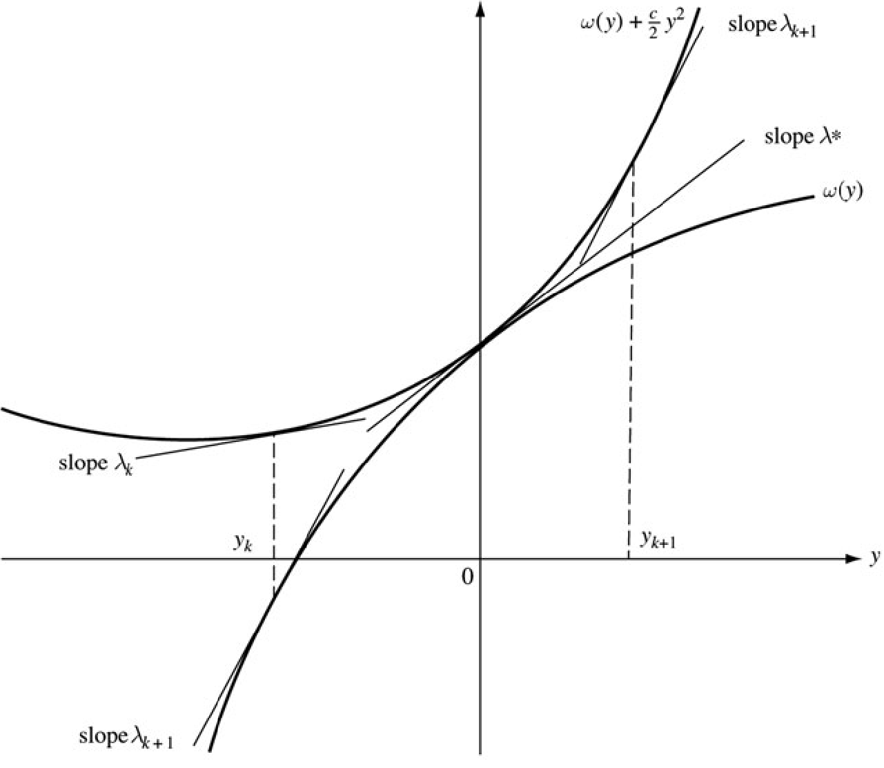
• The minimum of the augmented Lagrangian at step $k$ can be expressed in terms of the primal function as follows:

$$\begin{align} \operatorname{min} \ell_c(\bm{x}, \bm{\lambda}_k) &= \operatorname{min}_\bm{x} \left\{ f(\bm{x}) - \bm{\lambda}_k^\top \bm{h}(\bm{x}) + \frac{1}{2}c\left|\bm{h}(\bm{x})\right|^2 \right\} \\ &= \operatorname{min}_{\bm{x}, \bm{y}} \left\{ f(\bm{x}) - \bm{\lambda}_k^\top \bm{y} + \frac{1}{2}c|\bm{y}|^2: \, \bm{h}(\bm{x}) = \bm{y} \right\} \\ &= \operatorname{min}_\bm{y} \left\{ \omega(\bm{y}) - \bm{\lambda}_k^\top \bm{y} + \frac{1}{2}c|\bm{y}|^2 \right\}, \end{align}$$

where the minimization with respect to $\bm{y}$ is taken to be locally near $\bm{y} = \bm{0}$.

• In general, if $\bm{x}(\bm{\lambda_k})$ minimizes $\ell_c(\bm{x}, \bm{\lambda}_k)$, then $\bm{y}_k = \bm{h}(\bm{x}(\bm{\lambda_k}))$ is the minimum of $\omega(\bm{y}) - \bm{\lambda}_k^\top \bm{y} + \frac{1}{2}c|\bm{y}|^2$.
  • At that point we have $$\begin{align} &\nabla \omega (\bm{y}_k)^\top + c\bm{y}_k = \bm{\lambda}_k \\ &\nabla \omega(\bm{y}_k)^\top = \bm{\lambda}_k - c \bm{y}_k = \bm{\lambda}_k - c \bm{h}(\bm{x}(\bm{y}_k)). \end{align}$$
• It follows that for the next multiplier we have $$\bm{\lambda}_{k+1} = \bm{\lambda}_k - c\bm{h}(\bm{x}(\bm{\lambda}_k)) = \nabla \omega (\bm{y}_k)^\top.$$

Primal function

$$\omega(\bm{y}) \triangleq \operatorname{min}\left\{ f(\bm{x}): \bm{h}(\bm{x}) = \bm{y} \right\},$$ where the minimum is understood to be taken locally near $\bm{x}^\ast$.

• $\omega(\bm{0}) = f(\bm{x}^\ast)$.
• $\nabla \omega(\bm{0})^\top = \bm{\lambda}^\ast$.

Alternating Direction Method of Multipliers

Problem Set-Up

• Consider the convex minimization model with linear/affine constraints and an objective function that is the sum of two separable functions with two blocks of variables:

$$\begin{align} \operatorname{minimize} & f_1(\bm{x}^1) + f_2(\bm{x}^2), & f_i: \mathbb{R}^{n_i} \rightarrow \mathbb{R}, \\ \text{subject to} & \bm{A}_1 \bm{x}^1 + \bm{A}_2 \bm{x}^2 = \bm{b}, & \bm{b} \in \mathbb{R}^m \\ & \bm{x}^1 \in \Omega_1, \; \bm{x}^2 \in \Omega_2 & \Omega_i \subseteq \mathbb{R}^{n_i} \end{align} \qquad(14)$$

• Then, the augmented Lagrangian function for Equation 14 would be $$\ell_c(\bm{x}^1, \bm{x}^2, \bm{\lambda}) = f_1(\bm{x}^1) + f_2(\bm{x}^2) - \bm{\lambda}^\top \left(\bm{A}_1\bm{x}^1 + \bm{A}_2\bm{x}^2 - \bm{b} \right) + \frac{c}{2} \left| \bm{A}_1\bm{x}^1 + \bm{A}_2\bm{x}^2 - \bm{b} \right|^2.$$

• In contrast to the method of multipliers that we previously covered, the alternating direction method of multipliers (ADMM) is to (approximately) minimize $\ell_c(\bm{x}^1, \bm{x}^2, \bm{\lambda})$ in an alternative order:

$$\begin{align} \bm{x}_{k+1}^1 &:= \operatorname{arg}\operatorname{min}_{\bm{x}^1 \in \Omega_1} \ell_c(\bm{x}^1, \bm{x}_k^2, \bm{\lambda}_k), \\ \bm{x}_{k+1}^2 &:= \operatorname{arg}\operatorname{min}_{\bm{x}^2 \in \Omega_2} \ell_c(\bm{x}_{k+1}^1, \bm{x}^2, \bm{\lambda}_k), \\ \bm{\lambda}_{k+1} &:= \bm{\lambda}_k - c\left( \bm{A}_1\bm{x}_{k+1}^1 + \bm{A}_2\bm{x}_{k+1}^2 - \bm{b} \right). \end{align}$$

• The idea is that each of the smaller-block minimization problems can be solved more efficiently or even in closed-forms for certain cases.