Optimization Theory and Practice

---

Unconstrained Optimization

Instructor: Hasan A. Poonawala

Mechanical and Aerospace Engineering
University of Kentucky, Lexington, KY, USA

Topics:
Solutions
Necessary and Sufficient Conditions
Overview of Algorithms

Example: Curve Fitting

Suppose we have data in the form of pairs $$\{t_{i},y_{i}\}_ {i \in \{1,\dots,m\}}.$$

We believe that the model is of the form $$\phi(t; \theta) = \theta_{1} + \theta_{2} e^{\frac{(\theta_{3}-t )^2}{\theta_{4}}} + \theta_{5} \cos(\theta_{6} t).$$

A standard approach is to find the values of $\theta_{j}$, $j \in \{1,\dots,6\}$ by solving $$\min_{\theta \in \mathbb R^6} \sum_{j=1}^{6} r_{i}^{2}(\theta)$$ where $$r_{i}(\theta) = y_{i} - \phi(t_{i}; \theta)$$

This is a nonlinear least-square problem.

Solutions

Global minimizer

A point $x^{*}$ is a global minimizer if $f(x^*) \leq f(x)$ for all $x \in \mathbb R^n$.

Local minimizer

A point $x^{*}$ is a local minimizer if there is a neighborhood $\mathcal N$ of $x^*$ where $f(x^*) \leq f(x)$ for all $x \in \mathcal N$, where a neighborhood of $y$ is an open set containing $y$.

Strict local minimizer

A point $x^{*}$ is a strict local minimizer if there is a neighborhood $\mathcal N$ of $x^*$ where $f(x^*) < f(x)$ for all $x \in \mathcal N$ with $x \neq x^*$.

Taylor’s theorem

Taylor’s Theorem

Suppose that $f \colon \mathbb R^n \to \mathbb R$ is continuously differentiable and that $p \in \mathbb{R}^n$. Then we have that $$f(x+p) = f(x) + \nabla f(x+t p) p$$ for some $t \in (0,1)$. Moreover, if $f$ is twice continuously differentiable, we have that $$\nabla f(x+p) = \nabla f(x) + \int_{0}^{1} \nabla^2 f(x+t p) p dt$$ and that $$f(x+p) = f(x) + \nabla f(x) p + \frac{1}{2} p^T \nabla^2 f(x+t p) p$$ for some $t \in (0,1)$.

First-order Necessary Condition

FONC

If $x^{\star}$ is a local minimizer and $f$ is continuously differentiable in an open neighborhood of $x^{\star}$, then $\nabla f (x^{\star}) = 0$.

Notice that this is not the same as $\nabla f (x^{\star}) = 0 \implies x^{\star}$ is a local minimizer

Stationary point

A point $x^{\star}$ is a stationary point if it satisfies $\nabla f(x^{\star})=0$

Second-order Necessary Condition

SONC

If $x^{\star}$ is a local minimizer of $f$ and $\nabla^2 f$ exists and is continuous in an open neighborhood of $x^{\star}$, then $\nabla f (x^{\star}) = 0$ and $\nabla^2 f (x^{\star})$ is positive semidefinite.

Positive semidefinite matrix

A matrix $M$ is positive semidefinite, denoted¹ $M \succeq 0$, if $$x ^T M x \geq 0\quad \forall x \in \mathbb{R}^n.$$

If $M = H^T H$ for some real matrix $H$, then $M$ is positive semidefinite.

1. or sometimes $M \geq 0$

Second-order Sufficient Condition

SOSC

Suppose that $\nabla^2 f (x^{\star})$ is continuous in a neighborhood of $x^{\star}$ and that $\nabla f (x^{\star}) = 0$ and $\nabla^2 f (x^{\star})$ is positive definite. Then $x^{\star}$ is a strict local minimizer of $f$.

Positive definite matrix

A matrix $M$ is positive definite, denoted¹ $M \succ 0$, if $$x ^T M x > 0\quad \forall x \in \mathbb{R}^n,\ x \neq 0.$$

1. or sometimes $M > 0$

First-order Sufficient Condition

There is no first-order sufficient condition for $f$ when it is only differentiable

However, when $f$ is also convex, there is.

Convex functions

A function $f \colon \mathcal D \to \mathbb R$ is convex if $\mathcal D$ is a convex set and f $$f( \lambda x + (1-\lambda) y) \leq \lambda f(x) + (1-\lambda) f(y)$$ for all $x,y \in \mathcal D$ and $\lambda \in [0,1]$.

FOSC for convex $f$

When $f$ is convex, any local minimizer $x^{\star}$ is a global minimizer of $f$ . If in addition $f$ is differentiable, then any stationary point $x^{\star}$ is a global minimizer of $f$.

Summary

Condition	What we know	What it tells us	Notes
1st Ord Necessary	$x^\star$ is LM1, $f$ differentiable	$\nabla f(x^{\star})=0$	Proof justifies steepest descent
2nd Ord Necessary	$x^\star$ is LM, $f$ and $\nabla^2 f$ exist, are continuous on $\mathcal N$	$\nabla f(x^{\star})=0$ and $\nabla^2 f(x^{\star})$ is PSD
2nd Ord Sufficient	$\nabla f(x^{\star})=0$ and $\nabla^2 f(x^{\star})$ is PD	$x^\star$ is strict LM	Leads to algorithms for finding LMs
1st Ord Sufficient	$f$ is convex, $x^\star$ is LM	$x^\star$ is GM2
1st Ord Sufficient	$f$ is convex, differentiable, $\nabla f(x^{\star})=0$	$x^\star$ is GM	Leads to effective algorithms for finding global minima

1. Local Minimizer

2. Global Minimizer

Overview of Algorithms

• Recall that the algorithms are iterative
• We need a starting point $\mathbf x_0$
• … and a method to produce iterates $\mathbf{x}_1$, $\mathbf{x}_2$,$\dots$
• Generally two methods:
  • Line Search
  • Trust Region

Note

The words method and algorithm are used interchangeably

Line Search Methods

• The algorithm chooses a direction $p_k \in \mathbb{R}^n$
• Then, minimize $f(x)$ on the line defined by $\mathbf{x}_k + \alpha p_k$. That is, solve $$\min_{\alpha>0}\quad f(\mathbf{x}_k + \alpha p_k) \qquad(1)$$
  • In practice choose an $\alpha$ that makes $f(\mathbf{x}_{k+1}) < f(\mathbf{x}_{k})$, not solve Equation 1.
  • Practical method uses back-tracking line search to pick $\alpha$ given $p_k$

Line Search Methods

• Two common choices for directions.
  • Negative gradient (steepest descent) $$p_k = - \nabla f(\mathbf{x}_{k})$$
  • Newton direction: $$p_k = - (\nabla^2 f(\mathbf{x}_{k}))^{-1}\nabla f(\mathbf{x}_{k})$$

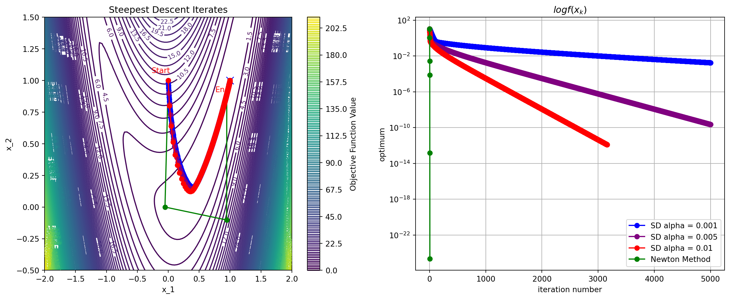
Example: Line Search Algorithms

$$\begin{align} \operatorname{minimize} & f(x) = (0.5 x_1 - 2)^2 + (x_2 - 3)^2 \end{align}$$

Important

Newton’s method is not always better

Plotting Code

import numpy as np
import matplotlib.pyplot as plt

# Define the objective function and its gradient and Hessian
def f(x, y):
    return #<answer>

def grad_f(x, y):
    """Gradient of f"""
    return np.array()

def hess_f(x, y):
    """Hessian of f"""
    return np.array()


# Steepest Descent
def steepest_descent(start, alpha=0.1,tol=1e-6, max_iter=50):
    # your code
    return x, iterates


# Plotting
x = np.linspace(-1, 4, 100)
y = np.linspace(-1, 5, 100)
X, Y = np.meshgrid(x, y)
Z = f(X, Y)

plt.figure(figsize=(8, 6))
# Contour plot of the objective function
contour = plt.contour(X, Y, Z, levels=30, cmap="viridis")
plt.clabel(contour, inline=True, fontsize=8)
plt.colorbar(contour, label="Objective Function Value")

plt.plot(4, 3, 'x', color="blue", markersize=10, label="True Optimum (4, 3)")

# Run Steepest Descent
start_point = [-1.0, 1.0]
optimum, iterates = steepest_descent(start_point)
# Extract iterate points for plotting
iterates = np.array(iterates)
x_iterates, y_iterates = iterates[:, 0], iterates[:, 1]
plt.plot(x_iterates, y_iterates, 'o-', color="blue", label="SD Iterates alpha=0.1")

# Annotate start and end points
plt.annotate("Start", (x_iterates[0], y_iterates[0]), textcoords="offset points", xytext=(-10, 10), ha="center", color="red")
plt.annotate("End", (x_iterates[-1], y_iterates[-1]), textcoords="offset points", xytext=(-10, -15), ha="center", color="red")

# Labels and legend
plt.xlabel("x_1")
plt.ylabel("x_2")
plt.title("Steepest Descent vs Newton's Method for Optimization")
plt.legend()
plt.grid(True)
plt.show()

Trust Region Methods

• Approximate $f$ near $\mathbf{x}_k$ using a model function $m_k$
• Minimize $m_k$ near $\mathbf{x}_k$ by solving $$\begin{align} \min_{p} & m_k\left(\mathbf{x}_k+p\right)\\ \text{s.t.} & \mathbf{x}_k+p \in \text{Trust region} \end{align}$$
• Common choice: local quadratic Taylor series, with a spherical trust region
  (trust-region Newton’s method)

Line Search and Trust Region Methods

In some cases, the two methods overlap ¹ $$\begin{align} \min_{p} & m_k\left(\mathbf{x}_k+p\right) = f_K + p^T \nabla f_k\\ \text{s.t.} & \| p\|_2 \leq \alpha \| \nabla f_k\|_2 \end{align}$$yields $$p = - \alpha \nabla f_{k}$$

1. $f_k = f(\mathbf{x}_k)$, $\nabla f_k = \nabla f(\mathbf{x}_k)$

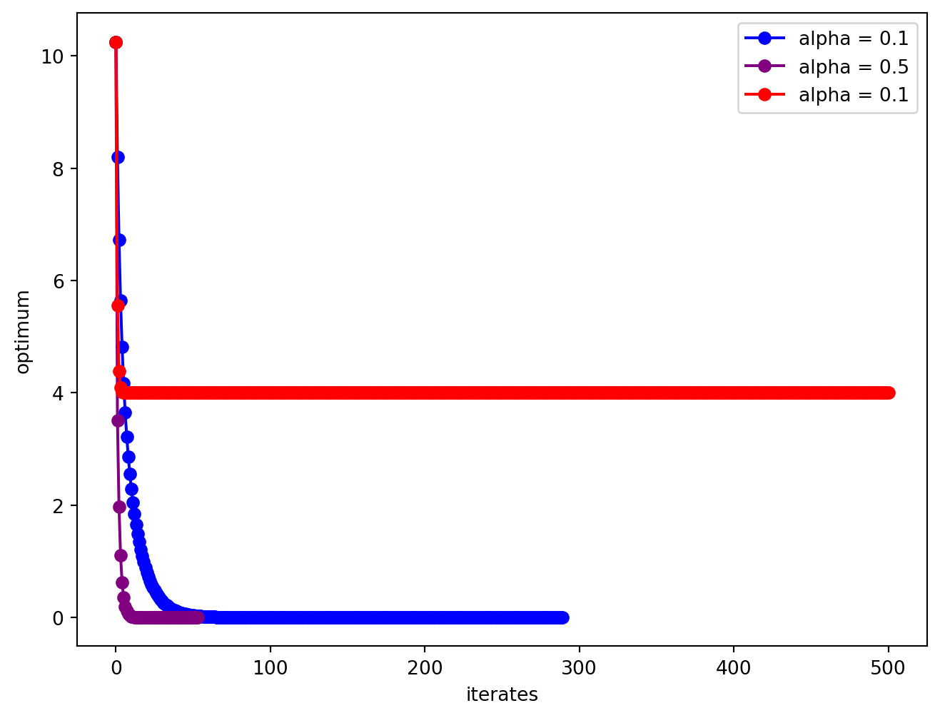
Exercise: Steepest Descent

$$\begin{align} \operatorname{minimize} & f(x) = (1 - x_1)^2 + 10 (x_2 - x_1^2)^2 \end{align}$$

The optimum is at $(1,1)$. Test the behavior of steepest descent algorithms $x_{k+1} = x_{k} - \alpha \nabla f_k$ with various constant values of $\alpha$, starting from $(0,1)$.

Solution

$$\nabla f = \begin{bmatrix} -2(1-x_1) - 40 (x_2 - x_1^2) x_1\\ 20 (x_2-x_2^2)\end{bmatrix}$$