Iterative LQR (iLQR)

---

Line Search, Forward Pass, and Full Algorithm

Instructor: Hasan A. Poonawala

Mechanical and Aerospace Engineering
University of Kentucky, Lexington, KY, USA

Topics:
Why $\alpha$ scales only $k_{t}$
Nonlinear forward pass
Backtracking line search
Full algorithm

Recap

The Setup

Nominal trajectory $\bar{x}_0, \bar{u}_0, \dots, \bar{x}_{T-1}, \bar{u}_{T-1}, \bar{x}_{T}, \bar{u}_{T-1}, \bar{x}_{T}$ satisfies the true nonlinear dynamics.

Define deviations: $\delta x_{t} = x_{t} - \bar{x}_{t}$, $\quad \delta u_{t} = u_{t} - \bar{u}_{t}$.

Linearized error dynamics around the nominal: $$\delta x_{t+1} \approx A_{t}\,\delta x_{t} + B_{t}\,\delta u_{t}, \qquad A_{t} = \left.\frac{\partial f}{\partial x}\right|_{\bar{x}_{t},\bar{u}_{t}}, \quad B_{t} = \left.\frac{\partial f}{\partial u}\right|_{\bar{x}_{t},\bar{u}_{t}}$$

Quadratic cost (second-order Taylor expansion of $c_{t}$ around nominal):

$$c_{t} \approx \bar{c}_{t} + \begin{bmatrix}q_{t} \\ r_{t}\end{bmatrix}^{\!T} \begin{bmatrix}\delta x \\ \delta u\end{bmatrix} + \frac{1}{2}\begin{bmatrix}\delta x \\ \delta u\end{bmatrix}^{\!T} \begin{bmatrix} Q_t^{cost} & S_t^{\!T} \\ S_t & R_t\end{bmatrix}\begin{bmatrix}\delta x \\ \delta u\end{bmatrix}$$

Unlike LQR, the linear terms $q_t$ and $r_t$ are generally nonzero — the nominal is not yet optimal.

Backward Pass: Q-function

The Q-function for the deviation problem:

$$\tilde{Q}_{t}(\delta x, \delta u) \approx \text{const} + \begin{bmatrix}\hat{q}_x \\ \hat{q}_u\end{bmatrix}^{\!T} \begin{bmatrix}\delta x \\ \delta u\end{bmatrix} + \frac{1}{2}\begin{bmatrix}\delta x \\ \delta u\end{bmatrix}^{\!T} \begin{bmatrix}\hat{Q}_{xx} & \hat{Q}_{xu} \\ \hat{Q}_{ux} & \hat{Q}_{uu}\end{bmatrix}\begin{bmatrix}\delta x \\ \delta u\end{bmatrix}$$

Backward recursion (initialize $\mathbf{v}_{T} = \mathbf{c}_{T}$, $\mathbf{V}_{T} = \mathbf{C}_{T}$):

$$\hat{q}_x = q_t + A_{t}^T \mathbf{v}_{t+1}, \qquad \hat{q}_u = r_t + B_{t}^T \mathbf{v}_{t+1}$$ $$\hat{Q}_{xx} = Q_t^{cost} + A_{t}^T \mathbf{V}_{t+1} A_{t}, \quad \hat{Q}_{uu} = R_t + B_{t}^T \mathbf{V}_{t+1} B_{t}, \quad \hat{Q}_{ux} = S_t + B_{t}^T \mathbf{V}_{t+1} A_{t}$$

Backward Pass: Optimal Gains

Minimize $\tilde{Q}_{t}$ over $\delta u$ (holding $\delta x$ fixed): $$\frac{\partial \tilde{Q}_{t}}{\partial \,\delta u} = \hat{q}_u + \hat{Q}_{uu}\,\delta u + \hat{Q}_{ux}\,\delta x = 0$$

$$\implies \delta u_{t}^* = \underbrace{-\hat{Q}_{uu}^{-1} \hat{q}_u}_{k_{t}} + \underbrace{(-\hat{Q}_{uu}^{-1} \hat{Q}_{ux})}_{K_{t}}\,\delta x_{t}$$

Gain	Expression	Role
$k_{t} \in \mathbb{R}^m$	$-\hat{Q}_{uu}^{-1} \hat{q}_u$	Feedforward — optimization step
$K_{t} \in \mathbb{R}^{m \times n}$	$-\hat{Q}_{uu}^{-1} \hat{Q}_{ux}$	Feedback — state-dependent correction

Value function updated as: $\mathbf{v}_{t} = \hat{q}_x + \hat{Q}_{xu} k_{t}$, $\quad \mathbf{V}_{t} = \hat{Q}_{xx} + \hat{Q}_{xu} K_{t}$

At the optimum $\hat{q}_u = r_t + B_{t}^T \mathbf{v}_{t+1} = 0$, so $k_{t} = 0$ — identical to LQR.

Forward Pass

The Forward Pass Update

Starting from $\hat{x}_0 = \bar{x}_0$¹, for $t = 0, 1, \dots, T-1$:

$$\boxed{\hat{u}_{t} = \bar{u}_{t} + \alpha\, k_{t} + K_{t}\underbrace{(\hat{x}_{t} - \bar{x}_{t})}_{\delta x_{t}}}$$ $$\hat{x}_{t+1} = f\!\left(\hat{x}_{t},\; \hat{u}_{t}\right) \qquad \leftarrow \text{true nonlinear dynamics}$$

Discussion: $\alpha$ multiplies $k_{t}$ but not $K_{t}$. Shouldn’t we scale the entire update $\delta u_{t} = \alpha(k_{t} + K_{t} \delta x_{t})$?

1. $\hat{x}$ is the updated nominal value (originally $\bar{x}$) of $x$

Line Search

Backtracking Line Search

Goal: find $\alpha \in (0, 1]$ such that the updated trajectory strictly reduces cost.

Algorithm:

1. Set $\alpha = 1$
2. Run nonlinear forward pass with current $\alpha$; evaluate $J(\hat{u})$
3. If $J(\hat{u}) < J(\bar{u})$: accept, update $\bar{x} \leftarrow \hat{x}$, $\bar{u} \leftarrow \hat{u}$
4. Else: $\alpha \leftarrow \alpha/2$, repeat from step 2
5. After 50 halvings: if $\alpha < 2\times 10^{-6}$, declare convergence

alpha = 1.0
for _ in range(50):
    for t in range(T):
        delta_u = K[t] @ (x_new[t] - x_nom[t]) + alpha * k_ff[t]
        u_new[t] = u_nom[t] + delta_u
        x_new[t+1] = f(x_new[t], u_new[t])   # nonlinear step
    if new_cost < current_cost:
        break
    alpha *= 0.5

Predicted Cost Improvement

The backward pass implicitly computes the predicted improvement:

$$\Delta J = \sum_{k=0}^{T-1}\left(\hat{q}_u^T k_{t} + \frac{1}{2} k_{t}^T \hat{Q}_{uu} k_{t}\right) = -\frac{1}{2}\sum_{k=0}^{T-1} k_{t}^T \hat{Q}_{uu} k_{t} \;\leq\; 0$$

This motivates a stronger Armijo condition:

$$J(\hat{u}) < J(\bar{u}) - \gamma\,\alpha\,|\Delta J|, \qquad \gamma \in (0,1)$$

Actual decrease must be at least a fraction $\gamma$ of the quadratic model’s prediction.

At convergence: $k_{t} \to 0$ (because $\hat{q}_u \to 0$), so $\Delta J \to 0$ and $\alpha = 1$ is accepted immediately on the first try — the line search costs nothing.

iLQR: Complete Algorithm

iLQR

Input: initial controls $\bar{u}_{0:T-1}$, dynamics $f_{t}$, costs $c_{t}$, $c_{T}$

1. Rollout: simulate $\bar{x}_{t+1} = f_{t}(\bar{x}_{t}, \bar{u}_{t})$ to obtain the nominal trajectory.

2. Repeat until convergence:

2a. Backward pass — init $\mathbf{v}_{T} = \mathbf{c}_{T}$, $\mathbf{V}_{T} = \mathbf{C}_{T}$; for $t = T-1, \dots, 0$:

• Compute Jacobians $A_{t}, B_{t}$ and cost derivatives at $(\bar{x}_{t}, \bar{u}_{t})$
• Compute $\hat{q}_x, \hat{q}_u, \hat{Q}_{xx}, \hat{Q}_{uu}, \hat{Q}_{ux}$ via the recursion
• Gains: $k_{t} = -\hat{Q}_{uu}^{-1} \hat{q}_u$, $\quad K_{t} = -\hat{Q}_{uu}^{-1} \hat{Q}_{ux}$
• Update: $\mathbf{v}_{t} = \hat{q}_x + \hat{Q}_{xu} k_{t}$, $\quad \mathbf{V}_{t} = \hat{Q}_{xx} + \hat{Q}_{xu} K_{t}$

2b. Forward pass — from $\hat{x}_0 = \bar{x}_0$, simulate with $\hat{u}_{t} = \bar{u}_{t} + \alpha k_{t} + K_{t}(\hat{x}_{t} - \bar{x}_{t})$

2c. Line search — if $J(\hat{u}) < J(\bar{u})$: accept; else $\alpha \leftarrow \alpha/2$, repeat 2b

2d. Update — $\bar{x}_{t} \leftarrow \hat{x}_{t}$, $\;\bar{u}_{t} \leftarrow \hat{u}_{t}$

iLQR vs. LQR

Quantity	LQR	iLQR (per iteration)
Dynamics	$x_{t+1} = A_{t} x_{t} + B_{t} u_{t}$	$\delta {x}_{t+1} = A_{t} \delta x_{t} + B_{t} \delta u_{t}$
Cost	Quadratic in $(x, u)$	Quadratic in $(\delta x, \delta u)$; linear terms nonzero
$\hat{Q}_{uu}$	$R + B^T P B$	$c_{uu} + B^T V_{xx} B$
Optimal control	$u^* = -K x$	$\delta u^* = k + K \delta x$
Feedforward	None ($\hat{q}_u = 0$ at optimum)	$k = -\hat{Q}_{uu}^{-1} \hat{q}_u$ (drives improvement)
Hessian recursion	Discrete Riccati equation	Same Schur complement form

The backward pass is structurally identical to LQR applied to the deviation problem. The only additions: (1) feedforward gains $k_{t}$ from nonzero cost gradients; (2) re-linearize each iteration.

Demo: Iterates

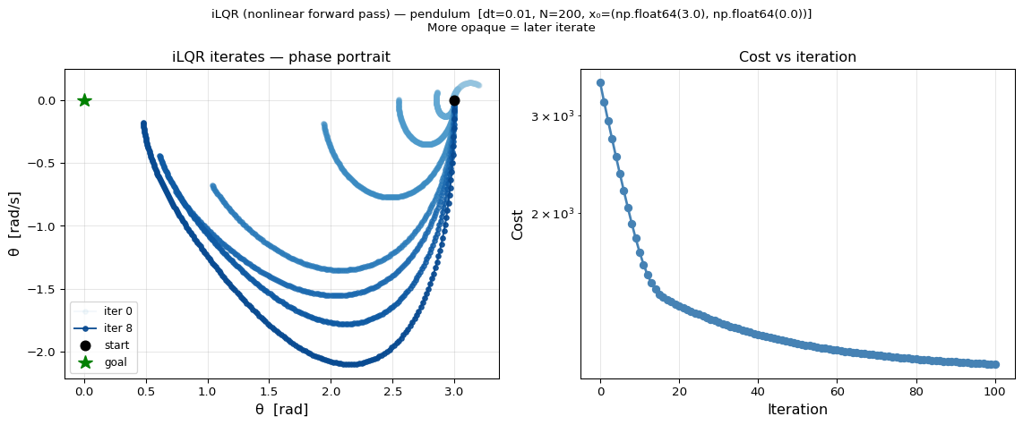
Pendulum swing-up from $\theta_0 = 3.0$ rad, $T = 200$ steps. Snapshots at iterations 0, 1, 2, 4, 8, 15, 25, 50, 100 (darker = later).

Extensions

Beyond iLQR

Differential Dynamic Programming (DDP):

iLQR uses only first-order Jacobians of $f_{t}$. DDP adds second-order terms:

$$\hat{Q}_{xx} \mathrel{+}= \sum_i (\mathbf{v}_{t+1})^{(i)} f_{t,xx}^{(i)}, \quad \hat{Q}_{uu} \mathrel{+}= \cdots, \quad \hat{Q}_{ux} \mathrel{+}= \cdots$$

• Terms scale as $\mathcal{O}(\|\mathbf{v}_{t+1}\|)$ — vanish near the optimum where $\mathbf{v}_{t+1} \to 0$
• Better convergence rate far from the optimum; expensive and rarely used in practice
• iLQR is sometimes called Gauss-Newton DDP

Beyond iLQR

Natural extensions:

Extension	Idea
Constrained iLQR	Handle $u_{t} \in \mathcal{U}$ via augmented Lagrangian (AL-iLQR)
MPC	Re-solve at each timestep with a receding horizon
Warm-starting	Initialize next solve from the shifted previous solution

Summary

Forward pass update: $$\hat{u}_{t} = \bar{u}_{t} + \alpha\, k_{t} + K_{t}(\hat{x}_{t} - \bar{x}_{t}), \qquad \hat{x}_{t+1} = f(\hat{x}_{t}, \hat{u}_{t})$$

• $\alpha$ scales only $k_{t}$ — the Newton search direction in $u$
• $K_{t} \delta x_{t}$ corrects for nonlinear drift
• Using nonlinear dynamics keeps the trajectory feasible at every iteration

Line search: halve $\alpha$ until $J$ decreases; $k_{t} \to 0$ signals convergence

Convergence ↔︎ optimality: $\hat{q}_u = 0$ is the discrete-time PMP stationarity condition

DDP vs. iLQR: dynamics Hessian terms improve convergence rate but are rarely worth the cost