LiDAR Inertial Odometry


Frame Transformations and Sensor Fusion


Instructor: Hasan A. Poonawala

Mechanical and Aerospace Engineering
University of Kentucky, Lexington, KY, USA

Topics:
Coordinate Frames
IMU and Wheel Odometry
Sensor Fusion for LIO

Lesson Overview

  1. Frame Transformations: Body, sensor, and world frames
  2. IMU Fundamentals: Accelerometers, gyroscopes, and integration
  3. Wheel Odometry: Encoders and kinematic models
  4. Sensor Fusion: Combining LiDAR with inertial/wheel data

Connection: Extends scan matching with additional sensors for robust odometry

Part 1: Coordinate Frames

Why Multiple Frames?

A mobile robot system involves several coordinate frames:

  • World frame \(\{W\}\): Fixed reference (e.g., room corner, starting position)
  • Body frame \(\{B\}\): Attached to robot chassis
  • LiDAR frame \(\{L\}\): Origin at LiDAR sensor
  • IMU frame \(\{I\}\): Origin at IMU sensor
  • Camera frame \(\{C\}\): If vision is used

Each sensor reports measurements in its own frame!

Frame Transformation Diagram


Transformation Notation

We use \(T_{AB}\) to denote the transformation from frame \(B\) to frame \(A\):

\[ \mathbf{p}^A = T_{B}^{A} \, \mathbf{p}^B \]

where \(\mathbf{p}^A\) is a point expressed in frame \(A\), and \(\mathbf{p}^B\) is the same point in frame \(B\).

Tip

Reading convention: \(T_{B}^{A}\) “takes points from \(B\) to \(A\)

Transformation Composition

Transformations chain naturally:

\[ T_{C}^{A} = T_{B}^{A} \cdot T_{C}^{B} \]

Example: Point in LiDAR frame to world frame

\[ \mathbf{p}^W = T_{B}^{W} \cdot T_{L}^{B} \cdot \mathbf{p}^L \]

The “inner” subscripts must match (like matrix dimensions)!

SE(2) Transformation Review

Recall from scan matching, in 2D:

\[ T = \begin{bmatrix} R(\theta) & \mathbf{t} \\ \mathbf{0}^T & 1 \end{bmatrix} = \begin{bmatrix} \cos\theta & -\sin\theta & t_x \\ \sin\theta & \cos\theta & t_y \\ 0 & 0 & 1 \end{bmatrix} \]

Inverse transformation: \[ T^{-1} = T_{A}^{B} = \begin{bmatrix} R^T & -R^T \mathbf{t} \\ \mathbf{0}^T & 1 \end{bmatrix} \]

Extrinsic Calibration

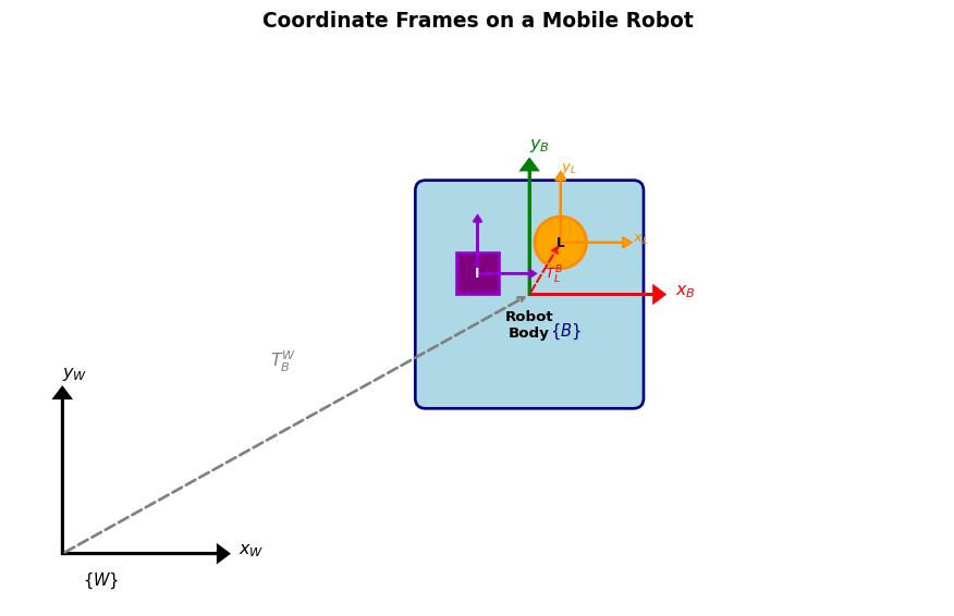
The transformation between rigidly mounted sensors is constant:

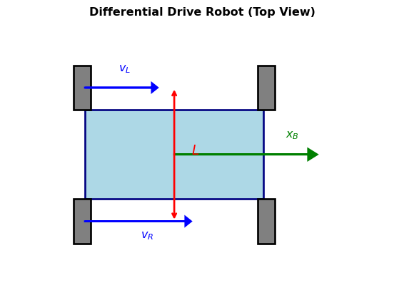
  • \(T_{L}^{B}\): LiDAR pose relative to body frame
  • \(T_{I}^{B}\): IMU pose relative to body frame

These are determined by extrinsic calibration:

  • Measure physical offsets and orientations
  • Or use calibration procedures (target-based, hand-eye calibration)

Warning

Calibration errors propagate through all subsequent computations!

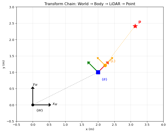
Example: LiDAR Point to World Frame

import numpy as np

def make_se2(theta, tx, ty):
    """Create SE(2) transformation matrix."""
    c, s = np.cos(theta), np.sin(theta)
    return np.array([[c, -s, tx], [s, c, ty], [0, 0, 1]])

# Extrinsic: LiDAR is 0.3m forward of body origin, aligned
T_BL = make_se2(0, 0.3, 0)

# Robot pose in world: at (2, 1) with 45° heading
T_WB = make_se2(np.pi/4, 2.0, 1.0)

# A point detected by LiDAR at (1.5, 0.2) in LiDAR frame
p_L = np.array([1.5, 0.2, 1])  # homogeneous

# Transform to world frame
p_W = T_WB @ T_BL @ p_L
print(f"Point in world frame: ({p_W[0]:.3f}, {p_W[1]:.3f})")
Point in world frame: (3.131, 2.414)

Visualizing the Transform Chain

Code
fig, ax = plt.subplots(figsize=(8, 6))

# World frame
ax.arrow(0, 0, 0.5, 0, head_width=0.08, head_length=0.05, fc='black', ec='black', lw=2)
ax.arrow(0, 0, 0, 0.5, head_width=0.08, head_length=0.05, fc='black', ec='black', lw=2)
ax.text(0.6, 0, r'$x_W$', fontsize=11)
ax.text(0, 0.6, r'$y_W$', fontsize=11)
ax.plot(0, 0, 'ko', markersize=8)
ax.text(0.1, -0.2, r'$\{W\}$', fontsize=10, fontweight='bold')

# Robot position and orientation
robot_pos = np.array([2.0, 1.0])
robot_theta = np.pi/4
R_WB = np.array([[np.cos(robot_theta), -np.sin(robot_theta)],
                 [np.sin(robot_theta), np.cos(robot_theta)]])

# Body frame axes
ax.arrow(robot_pos[0], robot_pos[1], 0.4*R_WB[0,0], 0.4*R_WB[1,0],
         head_width=0.08, head_length=0.05, fc='red', ec='red', lw=2)
ax.arrow(robot_pos[0], robot_pos[1], 0.4*R_WB[0,1], 0.4*R_WB[1,1],
         head_width=0.08, head_length=0.05, fc='green', ec='green', lw=2)
ax.plot(robot_pos[0], robot_pos[1], 'bs', markersize=12)
ax.text(robot_pos[0]+0.1, robot_pos[1]-0.25, r'$\{B\}$', fontsize=10, fontweight='bold', color='blue')

# LiDAR frame (0.3m forward in body frame)
lidar_offset_B = np.array([0.3, 0])
lidar_pos = robot_pos + R_WB @ lidar_offset_B
ax.arrow(lidar_pos[0], lidar_pos[1], 0.3*R_WB[0,0], 0.3*R_WB[1,0],
         head_width=0.06, head_length=0.04, fc='orange', ec='orange', lw=1.5)
ax.arrow(lidar_pos[0], lidar_pos[1], 0.3*R_WB[0,1], 0.3*R_WB[1,1],
         head_width=0.06, head_length=0.04, fc='orange', ec='orange', lw=1.5)
ax.plot(lidar_pos[0], lidar_pos[1], 'o', color='orange', markersize=10)
ax.text(lidar_pos[0]+0.15, lidar_pos[1]+0.1, r'$\{L\}$', fontsize=10, fontweight='bold', color='darkorange')

# Point in LiDAR frame
p_L_2d = np.array([1.5, 0.2])
p_W_2d = robot_pos + R_WB @ (lidar_offset_B + p_L_2d)
ax.plot(p_W_2d[0], p_W_2d[1], 'r*', markersize=15)
ax.text(p_W_2d[0]+0.1, p_W_2d[1]+0.1, r'$\mathbf{p}$', fontsize=12, color='red')

# Draw dashed lines showing the chain
ax.plot([0, robot_pos[0]], [0, robot_pos[1]], 'k--', alpha=0.3, lw=1)
ax.plot([robot_pos[0], lidar_pos[0]], [robot_pos[1], lidar_pos[1]], 'b--', alpha=0.3, lw=1)
ax.plot([lidar_pos[0], p_W_2d[0]], [lidar_pos[1], p_W_2d[1]], 'orange', ls='--', alpha=0.5, lw=1)

ax.set_xlim(-0.5, 4)
ax.set_ylim(-0.5, 3)
ax.set_aspect('equal')
ax.grid(True, alpha=0.3)
ax.set_xlabel('x (m)')
ax.set_ylabel('y (m)')
ax.set_title('Transform Chain: World → Body → LiDAR → Point')
plt.tight_layout()
plt.show()

Coordinate Transformation Vs Rigid Motion

Consider a robot with a center, a camera in ‘front’, and two wheels to the side.

Whenever we move the robot, the distances between these points don’t change.

As the robot moves, we can take a snapshot of these points, and they each define a coordinate frame for Euclidean space.

Coordinate Transformation Vs Rigid Motion (cont.)

Q1: How would the robot compare observations of either purple point over time?

A1: Coordinate transformations

Q2: How do we keep track of all the points on the robots?

A2: Coordinate transformations, but reinterpreted.

Coordinate Transformation Vs Rigid Motion (cont.)

We know how to express all points in the robot’s frame in any other frame: Use a distance-preserving coordinate transformation.

This transformation itself becomes a representative for all points on the robot.

We have seen that

\[p^B = \left(T_B^A\right)^{-1} \left(p^A - o_B^A\right)\]

Let \(d = o_B^A\) and \(R = T_B^A\).

From this, we can derive \[\begin{aligned} p^B & = {R}^{-1} \left(p^A - d\right) \\ p^{A} &= R\ p^{B} + d \end{aligned}\]

Rigid Body Pose

We refer to the pair \((d,R)\) as the pose – relative to frame \(A\) – of the rigid body to which frame \(B\) is attached.

Let’s reinterpret the two affine transformations associated with \((d,R)\). Consider vector \(v\) in frame \(A\):

\[\begin{aligned} \color{orange}{u_1} & = {R}^{-1} \left(v - d\right) & \text{ (Change of Basis)}\\ \color{green}{u_2} &= R\ v + d & \text{ (Rigid motion)} \end{aligned}\]

Rigid Body Pose: Visualization

  • If we view \(u_1\) as coordinates in frame \(B\), we’ve changed coordinates of \(v\) from world to body frame.
  • If we view \(u_2\) as coordinates in frame \(A\), we’ve moved the point \(o_A \oplus v\) relative to frame \(A\).

Rigid Body Pose (cont.)

The pair \((d,R) \in \mathbb{R}^3 \times \mathrm{SO}(3)\) tells us how to move points in frame \(A\) to achieve the same coordinates in frame \(B\).

\(d\) is a vector, the coordinates of origin of frame \(B\), and \(R\) is a matrix containing the coordinates of axes of \(B\), both relative to \(A\)

Move in frame \(A\) = reorient by \(R\) and then move by \(d\) : \(Rv+d\)

Example: Coordinate Transform vs Rigid Motion

  • Top row: Coordinate transform \(\left(R_B^A\right)^{-1}\) - fixed points in \(A\) seen by moving frame \(B\)
  • Bottom row: Rigid motion \(R_B^A\) - fixed points in moving frame \(B\) seen by fixed frame \(A\)

Special Euclidean Group \(\mathrm{SE}(3)\)

Important

Coordinates of points in 3D Euclidean space = \(p^A \in \mathbb{R}^3\)

Coordinates of cartesian frames in 3D Euclidean space = \((d,R) \in \mathrm{SE}(3) = \mathbb{R}^3 \times \mathrm{SO}(3)\)

Points : Euclidean Space :: Cartesian Frames : Special Euclidean Group

  • \(G\)-Torsor: A group \(G\) with an action that maps a group element to another group element

  • No coordinate frame is unique.

  • For \(\mathrm{SE}(3)\), a \(G\)-Torsor, we don’t define origin+basis (not a vector space).

  • Instead, we define an identity element (it’s a group): the reference coordinate frame.

Odometry: Sneak Peek

The Odometry Problem

Odometry: Estimate robot pose over time using onboard sensors

Given:

  • Sequence of sensor measurements \(z_1, z_2, \ldots, z_n\)
  • Initial pose \(T_{B_0}^{W}\) (often identity)

Find:

  • Pose at each time: \(T_{B_1}^{W}, T_{B_2}^{W}, \ldots, T_{B_n}^{W}\)

Scan Matching Odometry

From the previous lecture, ICP gives us relative pose between consecutive scans:

\[ T_{ B_{k+1}}^{B_{k}} \quad \text{(motion from time } k \text{ to } k+1\text{)} \]

Chain to get pose in world frame: \[ T_{ B_{k+1}}^{W} = T_{ B_k}^{W} \cdot T_{ B_{k+1}}^{B_k} \]

Warning

Problem: Errors accumulate! Small drift in each \(T_{ B_{k+1}}^{B_k}\) compounds over time.

Drift in LiDAR Odometry

Code
np.random.seed(42)

# Simulate a circular path with noisy odometry
n_steps = 100
true_radius = 5.0
true_poses = []
noisy_poses = []

# True circular motion
for i in range(n_steps):
    angle = 2 * np.pi * i / n_steps
    x = true_radius * np.cos(angle)
    y = true_radius * np.sin(angle)
    theta = angle + np.pi/2  # tangent direction
    true_poses.append([x, y, theta])

true_poses = np.array(true_poses)

# Simulate noisy relative measurements
T_accumulated = make_se2(0, true_radius, 0)  # Start at (5, 0)
noisy_poses.append([true_radius, 0, np.pi/2])

for i in range(1, n_steps):
    # True relative motion
    dx_true = true_poses[i, 0] - true_poses[i-1, 0]
    dy_true = true_poses[i, 1] - true_poses[i-1, 1]
    dtheta_true = true_poses[i, 2] - true_poses[i-1, 2]

    # Add noise (simulating scan matching error)
    dx = dx_true + np.random.normal(0, 0.01)
    dy = dy_true + np.random.normal(0, 0.01)
    dtheta = dtheta_true + np.random.normal(0, 0.005)

    # Relative transform in local frame
    T_rel = make_se2(dtheta, dx, dy)
    T_accumulated = T_accumulated @ T_rel

    noisy_poses.append([T_accumulated[0, 2], T_accumulated[1, 2],
                        np.arctan2(T_accumulated[1, 0], T_accumulated[0, 0])])

noisy_poses = np.array(noisy_poses)

fig, ax = plt.subplots(figsize=(8, 8))
ax.plot(true_poses[:, 0], true_poses[:, 1], 'g-', linewidth=2, label='Ground Truth')
ax.plot(noisy_poses[:, 0], noisy_poses[:, 1], 'r-', linewidth=2, label='Odometry (with drift)')
ax.plot(true_poses[0, 0], true_poses[0, 1], 'go', markersize=12, label='Start')
ax.plot(true_poses[-1, 0], true_poses[-1, 1], 'g^', markersize=12)
ax.plot(noisy_poses[-1, 0], noisy_poses[-1, 1], 'r^', markersize=12)

# Draw error
ax.annotate('', xy=(noisy_poses[-1, 0], noisy_poses[-1, 1]),
            xytext=(true_poses[-1, 0], true_poses[-1, 1]),
            arrowprops=dict(arrowstyle='<->', color='purple', lw=2))
#ax.text(-0.5, 6.5, 'Accumulated\nError', fontsize=11, color='purple')

ax.set_xlabel('x (m)')
ax.set_ylabel('y (m)')
ax.set_aspect('equal')
ax.grid(True, alpha=0.3)
ax.legend(loc='upper left')
ax.set_title('Odometry Drift: Robot Returns to Start but Estimate Does Not')
plt.tight_layout()
plt.show()

Part 2: IMU Fundamentals

Inertial Measurement Unit (IMU)

An IMU typically contains:

Accelerometer

  • Measures linear acceleration
  • 3-axis: \(a_x, a_y, a_z\)
  • Units: m/s²

Gyroscope

  • Measures angular velocity
  • 3-axis: \(\omega_x, \omega_y, \omega_z\)
  • Units: rad/s

Note

For 2D planar robots, we primarily use \(a_x\), \(a_y\) (in-plane) and \(\omega_z\) (yaw rate)

IMU Measurement Model

Gyroscope (simpler case): \[ \omega^{meas} = \omega^{true} + b_\omega + n_\omega \]

Accelerometer (includes gravity): \[ a^{meas} = R^T(a^{true} - g) + b_a + n_a \]

where:

  • \(b_{(\cdot)}\): slowly varying bias
  • \(n_{(\cdot)}\): white noise
  • \(g\): gravity vector (≈ 9.81 m/s² pointing down)
  • \(R\): Orientation of IMU-fixed frame relative to ground

Dead Reckoning with IMU

Given angular velocity \(\omega_z\) from gyroscope:

\[ \theta(t) = \theta_0 + \int_0^t \omega_z(\tau) \, d\tau \]

Discrete integration: \[ \theta_{k+1} = \theta_k + \omega_z \cdot \Delta t \]

Warning

Gyroscope bias causes linear drift in orientation over time!

Accelerometer Integration (2D Case)

For a planar robot, given accelerations \(a_x\), \(a_y\) in body frame:

Velocity integration: \[ \begin{aligned} v_x(t) &= v_{x,0} + \int_0^t a_x(\tau) \, d\tau \\ v_y(t) &= v_{y,0} + \int_0^t a_y(\tau) \, d\tau \end{aligned} \]

Position integration: \[ \begin{aligned} x(t) &= x_0 + \int_0^t v_x(\tau) \, d\tau \\ y(t) &= y_0 + \int_0^t v_y(\tau) \, d\tau \end{aligned} \]

The Double Integration Problem

Code
np.random.seed(123)

# Simulate IMU integration with bias
dt = 0.01
t = np.arange(0, 10, dt)
n = len(t)

# True motion: stationary
true_pos = np.zeros((n, 2))

# IMU with small bias
accel_bias = np.array([0.01, 0.005])  # m/s^2 bias
accel_noise_std = 0.1

# Integrate with bias
velocity = np.zeros((n, 2))
position = np.zeros((n, 2))

for i in range(1, n):
    # Measured acceleration (true = 0, but we have bias + noise)
    a_meas = accel_bias + accel_noise_std * np.random.randn(2)

    # Integrate
    velocity[i] = velocity[i-1] + a_meas * dt
    position[i] = position[i-1] + velocity[i] * dt

fig, axes = plt.subplots(1, 3, figsize=(12, 4))

axes[0].plot(t, position[:, 0], 'b-', label='Estimated x')
axes[0].plot(t, true_pos[:, 0], 'g--', label='True x', linewidth=2)
axes[0].set_xlabel('Time (s)')
axes[0].set_ylabel('Position (m)')
axes[0].set_title('X Position')
axes[0].legend()
axes[0].grid(True, alpha=0.3)

axes[1].plot(t, position[:, 1], 'r-', label='Estimated y')
axes[1].plot(t, true_pos[:, 1], 'g--', label='True y', linewidth=2)
axes[1].set_xlabel('Time (s)')
axes[1].set_ylabel('Position (m)')
axes[1].set_title('Y Position')
axes[1].legend()
axes[1].grid(True, alpha=0.3)

axes[2].plot(position[:, 0], position[:, 1], 'b-')
axes[2].plot(0, 0, 'go', markersize=10, label='True position')
axes[2].set_xlabel('x (m)')
axes[2].set_ylabel('y (m)')
axes[2].set_title('Estimated Trajectory (robot is stationary!)')
axes[2].legend()
axes[2].grid(True, alpha=0.3)
axes[2].set_aspect('equal')

plt.tight_layout()
plt.show()

print(f"After 10 seconds, position error: ({position[-1, 0]:.2f}, {position[-1, 1]:.2f}) m")
print(f"Bias: {accel_bias} m/s² → Position drift ≈ 0.5 * bias * t² = {0.5 * accel_bias[0] * 100:.2f} m")
After 10 seconds, position error: (0.46, 0.07) m
Bias: [0.01  0.005] m/s² → Position drift ≈ 0.5 * bias * t² = 0.50 m

IMU Drift Summary

Sensor Error Type Drift Rate
Gyroscope Orientation Linear in time (\(\propto t\))
Accelerometer Position Quadratic in time (\(\propto t^2\))

Important

IMU alone is unsuitable for long-term positioning, but excellent for short-term, high-frequency motion estimation!

Part 3: Wheel Odometry

Wheel Encoders

Wheel encoders measure rotation of robot wheels:

Encoder types:

  • Optical (common)
  • Magnetic
  • Hall effect

Output:

  • Ticks per revolution
  • Velocity or position

Resolution: Typical encoders have 100-10000+ counts per revolution

Differential Drive Kinematics

For a differential drive robot with wheel radius \(r\) and wheel separation \(L\):

Differential Drive Equations

Given left and right wheel velocities \(v_L\) and \(v_R\):

Linear velocity (at robot center): \[ v = \frac{v_R + v_L}{2} \]

Angular velocity: \[ \omega = \frac{v_R - v_L}{L} \]

From encoder ticks: \(v = r \cdot \dot{\phi}\) where \(\dot{\phi}\) is wheel angular velocity

Wheel Odometry Integration

Given \(v\) and \(\omega\) at each timestep:

\[ \begin{aligned} x_{k+1} &= x_k + v_k \cos(\theta_k) \cdot \Delta t \\ y_{k+1} &= y_k + v_k \sin(\theta_k) \cdot \Delta t \\ \theta_{k+1} &= \theta_k + \omega_k \cdot \Delta t \end{aligned} \]

Note

This assumes small \(\Delta t\) such that \(\theta\) is approximately constant during the interval

Wheel Odometry Implementation

def wheel_odometry(v_left, v_right, L, dt, x0=0, y0=0, theta0=0):
    """
    Compute odometry from wheel velocities.
    v_left, v_right: arrays of wheel velocities
    L: wheel separation
    dt: time step
    Returns: x, y, theta arrays
    """
    n = len(v_left)
    x, y, theta = np.zeros(n), np.zeros(n), np.zeros(n)
    x[0], y[0], theta[0] = x0, y0, theta0

    for k in range(n - 1):
        v = (v_right[k] + v_left[k]) / 2
        omega = (v_right[k] - v_left[k]) / L

        x[k+1] = x[k] + v * np.cos(theta[k]) * dt
        y[k+1] = y[k] + v * np.sin(theta[k]) * dt
        theta[k+1] = theta[k] + omega * dt

    return x, y, theta

Wheel Odometry Errors

Sources of error in wheel odometry:

  1. Wheel slip: Especially on smooth or uneven surfaces
  2. Wheel radius uncertainty: Manufacturing tolerance, tire pressure
  3. Encoder resolution: Quantization error
  4. Uneven terrain: Effective wheel separation changes

Tip

Wheel odometry is reliable on flat, indoor surfaces but degrades outdoors

Comparing Odometry Sources

Source Strengths Weaknesses
LiDAR (scan matching) No drift in feature-rich environments Fails in featureless areas, computationally heavy
IMU High frequency, no external dependencies Drifts quickly, needs calibration
Wheel encoders Simple, cheap, reliable indoors Slip, terrain-dependent

Key insight: Combine them for robust odometry!

Part 4: Sensor Fusion

Why Fuse Sensors?

Each sensor has complementary characteristics:

LiDAR-Inertial Odometry (LIO)

Core idea: Use IMU to provide:

  1. Motion prior for scan matching initialization
  2. High-frequency pose updates between LiDAR scans
  3. De-skewing of LiDAR scans (points collected during motion)

The IMU prevents scan matching from falling into local minima!

Basic LIO Pipeline

Motion Prior from IMU

Between LiDAR scans at times \(t_k\) and \(t_{k+1}\):

Integrate IMU measurements: \[ \hat{T}_{B_{k+1}, IMU}^{B_k} = \int_{t_k}^{t_{k+1}} (\omega, a) \, dt \]

Use as initial guess for ICP: \[ T_{B_{k+1}, init}^{B_k} = \hat{T}_{B_{k+1}, IMU}^{B_k} \]

This puts ICP in the basin of attraction of the correct solution!

Scan De-skewing

A single LiDAR scan takes time to complete (~50-100ms for 2D, more for 3D)

During this time, the robot moves → points are distorted

De-skewing: Use IMU to estimate pose at each point’s timestamp, then transform all points to a common frame

Code
np.random.seed(789)

# Simulate a scan during rotation
n_points = 100
scan_duration = 0.1  # 100ms scan
omega = 1.0  # rad/s rotation during scan

# Points on a wall at various angles
angles = np.linspace(0, np.pi, n_points)
ranges = 3.0 + 0.1 * np.random.randn(n_points)

# Time of each point measurement
t_points = scan_duration * np.linspace(0, 1, n_points)

# Distorted points (robot rotating during scan)
distorted_x = ranges * np.cos(angles + omega * t_points)
distorted_y = ranges * np.sin(angles + omega * t_points)

# Corrected points (de-skewed to start of scan)
corrected_x = ranges * np.cos(angles)
corrected_y = ranges * np.sin(angles)

fig, axes = plt.subplots(1, 2, figsize=(10, 5))

axes[0].scatter(distorted_x, distorted_y, c=t_points, cmap='viridis', s=20)
axes[0].set_title('Raw Scan (Skewed by Motion)')
axes[0].set_xlabel('x (m)')
axes[0].set_ylabel('y (m)')
axes[0].set_aspect('equal')
axes[0].grid(True, alpha=0.3)

axes[1].scatter(corrected_x, corrected_y, c=t_points, cmap='viridis', s=20)
axes[1].set_title('De-skewed Scan')
axes[1].set_xlabel('x (m)')
axes[1].set_ylabel('y (m)')
axes[1].set_aspect('equal')
axes[1].grid(True, alpha=0.3)

plt.colorbar(plt.cm.ScalarMappable(cmap='viridis'), ax=axes, label='Time (s)', shrink=0.8)
plt.tight_layout()
plt.show()

Simple Sensor Fusion: Complementary Filter

A lightweight approach for fusing gyroscope and scan matching orientations:

\[ \theta_{fused} = \alpha \cdot \theta_{scan} + (1 - \alpha) \cdot (\theta_{prev} + \omega_{gyro} \cdot \Delta t) \]

  • \(\alpha \approx 0.98\): Trust scan matching for low frequency, IMU for high frequency
  • Simple to implement, effective in practice
Code
def complementary_filter(theta_scan, theta_prev, omega_gyro, dt, alpha=0.98):
    """Fuse scan matching and gyroscope orientation estimates."""
    theta_gyro = theta_prev + omega_gyro * dt
    return alpha * theta_scan + (1 - alpha) * theta_gyro

Extended Kalman Filter (EKF)

A more principled approach for sensor fusion:

State: \(\mathbf{x} = [x, y, \theta, v, \omega, b_\omega, \ldots]^T\)

Predict (using IMU/wheel model): \[ \hat{\mathbf{x}}_{k+1|k} = f(\mathbf{x}_k, \mathbf{u}_k) \]

Update (using scan matching): \[ \mathbf{x}_{k+1|k+1} = \hat{\mathbf{x}}_{k+1|k} + K(\mathbf{z}_{scan} - h(\hat{\mathbf{x}}_{k+1|k})) \]

Modern LIO Systems

State-of-the-art LIO implementations:

  • LOAM (Lidar Odometry and Mapping): Edge and planar feature extraction
  • LIO-SAM: Factor graph optimization, tightly-coupled IMU
  • FAST-LIO2: Iterative Kalman filter, direct point cloud registration
  • Faster-LIO: Incremental voxel map for efficiency

These systems achieve centimeter-level accuracy over kilometer trajectories!

Frame Transformations in LIO

In a full LIO system, you must track:

  1. \(T_{B}^{W}(t)\): Body pose in world frame (the output!)
  2. \(T_{L}^{B}\): LiDAR extrinsics (calibrated once)
  3. \(T_{I}^{B}\): IMU extrinsics (calibrated once)

Every LiDAR point must be transformed: \[ \mathbf{p}^W = T_{B}^{W}(t) \cdot T_{L}^{B} \cdot \mathbf{p}^L \]

IMU measurements must account for lever arm if IMU is not at body origin!

Summary

  1. Frame transformations: Critical bookkeeping for multi-sensor systems

    • Use consistent notation: \(T_{B}^{A}\) takes points from \(B\) to \(A\)
    • Extrinsic calibration determines sensor-to-body transforms
  2. IMU: High frequency, short-term accurate, but drifts

    • Gyro drift is linear, accelerometer position drift is quadratic
  3. Wheel odometry: Simple and reliable indoors, suffers from slip

  4. Sensor fusion: Combine complementary sensors for robust odometry

    • IMU provides motion prior and enables scan de-skewing
    • LiDAR provides drift-free pose updates

References

  • Zhang, J. and Singh, S. “LOAM: Lidar Odometry and Mapping in Real-time” (RSS 2014)
  • Shan, T. et al. “LIO-SAM: Tightly-coupled Lidar Inertial Odometry via Smoothing and Mapping” (IROS 2020)
  • Xu, W. et al. “FAST-LIO2: Fast Direct LiDAR-Inertial Odometry” (T-RO 2022)
  • Barfoot, T. “State Estimation for Robotics” (Cambridge University Press)