Model Predictive Path Integral Control

---

MPPI: Sampling-Based Optimal Control

Instructor: Hasan A. Poonawala

Mechanical and Aerospace Engineering
University of Kentucky, Lexington, KY, USA

Topics:
From MPC to MPPI
Stochastic optimal control
Information-theoretic derivation
Importance sampling update
Algorithm and properties

A Progression in Optimal Control

Each method relaxes one key assumption of the previous.

Method	Dynamics	Key relaxation
LQR	linear	baseline: analytical solution
iLQR	nonlinear	drop linearity via local linearization
MPC	nonlinear	drop infinite horizon; add constraints; replan online
MPPI	nonlinear	drop differentiability; use sampling
PPO	unknown	drop the model entirely; learn from interaction

LQR → iLQR → MPC all require differentiable dynamics and cost. MPPI breaks that requirement.

When Gradient-Based MPC Struggles

iLQR and SQP-based MPC compute Jacobians and Hessians of $f$ and $\ell$ at every step.

This fails (or becomes fragile) when:

• The cost is non-smooth: binary collision indicators, distance-to-obstacle, contact forces
• The dynamics involve contact or discontinuities: legged robots, manipulation with grasping
• The dynamics are a black-box simulator: no analytical gradients available
• The cost landscape is highly non-convex: many local minima, gradient descent gets stuck

MPPI’s answer: replace gradient computation with parallel sampling.

Roll out many trajectories, weight them by cost, take the weighted average. No derivatives needed.

Modern GPUs can run thousands of trajectory simulations in parallel — making sampling practical within a real-time control loop.

Stochastic Optimal Control Problem Setup

System and Cost

Work in discrete time with a control-affine stochastic system:

$$x_{t+1} = f(x_t) + G(x_t)(u_t + \varepsilon_t), \qquad \varepsilon_t \sim \mathcal{N}(0, \Sigma)$$

where $G(x)$ is the control matrix (possibly state-dependent) and noise enters through the control channel.

The path cost over a horizon of $T$ steps is: $$S(\tau) = \phi(x_T) + \sum_{t=0}^{T-1} \ell(x_t, u_t)$$

with running cost decomposed as: $$\ell(x_t, u_t) = q(x_t) + \frac{1}{2} u_t^T R\, u_t$$

• $q(x)$: state-dependent cost — may be non-smooth, non-differentiable, or even binary
• $\frac{1}{2} u^T R u$: quadratic control penalty

Stochastic Optimal Control Problem

Goal is to minimize cost

$$min_{u_t} S(\tau)$$

Subject to

$$x_{t+1} = f(x_t) + G(x_t)(u_t + \varepsilon_t), \qquad \varepsilon_t \sim \mathcal{N}(0, \Sigma)$$

• Dynamics are control-affine with noise entering through control
• Cost is sum-of-stage-costs: $S(\tau) = \phi(x_T) + \sum_{t=0}^{T-1} \ell(x_t, u_t)$
• Stage cost $\ell$ has specific structure: $\ell(x_t, u_t) = q(x_t) + \frac{1}{2} u_t^T R\, u_t$

Information-Theoretic Reformulation

From Trajectory Optimization to Distribution Optimization

Rather than minimizing $S(\tau)$ directly, search over distributions $q(\tau)$ over trajectories.

Define the passive distribution $p_0(\tau)$: trajectories generated by rolling out the current nominal control sequence $v_{0:T-1}$ plus noise,

$$p_0(\tau) \propto \exp\!\left(-\frac{1}{2}\sum_t \varepsilon_t^T \Sigma^{-1} \varepsilon_t\right)$$

where $u_t = v_t + \varepsilon_t$ and $\varepsilon_t \sim \mathcal{N}(0, \Sigma)$.

Pose the information-theoretic optimal control problem:

$$\min_{q(\tau)} \quad \mathbb{E}_q[S(\tau)] + \lambda\, \mathrm{KL}(q \,\|\, p_0)$$

The two terms balance minimizing cost against staying close to the passive distribution.

Why the KL Term Is a Control Cost

For the control-affine system, the KL divergence between $q$ and $p_0$ is:

$$\mathrm{KL}(q \,\|\, p_0) = \frac{1}{2}\,\mathbb{E}_q\!\left[\sum_t \varepsilon_t^T \Sigma^{-1} \varepsilon_t\right]$$

Setting $R = \lambda \Sigma^{-1}$, the KL penalty becomes:

$$\lambda\,\mathrm{KL}(q \,\|\, p_0) = \frac{1}{2}\,\mathbb{E}_q\!\left[\sum_t \varepsilon_t^T R\, \varepsilon_t\right] = \mathbb{E}_q\!\left[\sum_t \frac{1}{2} u_t^T R\, u_t\right]$$

The information-theoretic problem is therefore equivalent to the original stochastic optimal control problem — no approximation yet.

This is the key structural observation: the KL regularizer and the quadratic control cost are the same thing, linked by $R = \lambda \Sigma^{-1}$.

Optimal Solution

The Gibbs Distribution

The variational problem

$$\min_{q(\tau)} \quad \mathbb{E}_q[S(\tau)] + \lambda\, \mathrm{KL}(q \,\|\, p_0)$$

has a closed-form solution. Taking the functional derivative $\delta/\delta q$ and setting to zero:

$$q^*(\tau) = \frac{1}{\eta}\, p_0(\tau) \exp\!\left(-\frac{S(\tau)}{\lambda}\right), \qquad \eta = \mathbb{E}_{p_0}\!\left[\exp\!\left(-\frac{S(\tau)}{\lambda}\right)\right]$$

This is the Gibbs (Boltzmann) distribution: it reweights the passive rollout distribution by an exponential of the negative cost.

• weight $\propto$ 1/cost

The temperature $\lambda$ controls the sharpness:

$\lambda$ small	$\lambda$ large
Greedy — concentrates on best trajectory	Diffuse — nearly uniform weights
Sharp selection	Exploration

Free Energy

The normalization constant $\eta$ has a direct interpretation. Substituting $q^*$ back:

$$\mathcal{F} = -\lambda \log \mathbb{E}_{p_0}\!\left[\exp\!\left(-\frac{S(\tau)}{\lambda}\right)\right]$$

This is the free energy — the minimum achievable value of the information-theoretic objective.

By Jensen’s inequality applied to the convex function $-\log$:

$$\mathcal{F} \leq \mathbb{E}_{p_0}[S(\tau)]$$

Optimal reweighting always improves over the passive (uncontrolled) rollout.

This mirrors the free energy in statistical mechanics, with $\lambda$ playing the role of temperature $k_B T$.

Control Update via Importance Sampling

From Optimal Distribution to Control

Given $q^*(\tau)$, the optimal control at time $t$ is:

$$u_t^* = v_t + \mathbb{E}_{q^*}[\varepsilon_t]$$

Using the definition of $q^*$ to convert to an expectation under $p_0$:

$$u_t^* = v_t + \frac{\mathbb{E}_{p_0}\!\left[\varepsilon_t \exp(-S/\lambda)\right]}{\mathbb{E}_{p_0}\!\left[\exp(-S/\lambda)\right]}$$

This is importance sampling: sample from $p_0$ (the easy distribution), reweight by $\exp(-S/\lambda)$.

No gradients of $f$ or $\ell$ appear anywhere in this expression. The dynamics and cost are treated as black boxes.

Monte Carlo Approximation

Approximate with $K$ samples $\varepsilon^{(k)} \sim p_0$:

$$u_t^* \approx v_t + \sum_{k=1}^{K} \tilde{w}^{(k)}\, \varepsilon_t^{(k)}, \qquad \tilde{w}^{(k)} = \frac{\exp(-S^{(k)}/\lambda)}{\sum_j \exp(-S^{(j)}/\lambda)}$$

The normalized weights $\tilde{w}^{(k)}$ sum to one and are higher for lower-cost trajectories.

Numerical stability: subtract $\beta = \min_k S^{(k)}$ before exponentiating:

$$w^{(k)} = \exp\!\left(-\frac{S^{(k)} - \beta}{\lambda}\right), \qquad \tilde{w}^{(k)} = \frac{w^{(k)}}{\sum_j w^{(j)}}$$

This is algebraically identical — $\beta$ cancels in the normalization — but prevents overflow.

When Is the Derivation Exact?

The derivation above is exact when:

1. Dynamics are control-affine with noise through the control channel: $x_{t+1} = f(x_t) + G(x_t)(u_t + \varepsilon_t)$
2. The control cost satisfies $R = \lambda \Sigma^{-1}$, so the KL term and control cost coincide

In practice, MPPI is applied more broadly:

• Non-affine dynamics (black-box simulators)
• Binary or discontinuous costs
• Constraints encoded as large penalties

The free-energy / importance-sampling structure is retained as a principled heuristic, but the optimality guarantee no longer holds exactly.

Even as a heuristic, MPPI consistently outperforms random shooting because the weighted average biases the update toward the low-cost region of trajectory space.

The Algorithm

MPPI

At each time step $t$ with current nominal control sequence $u_{t:t+N-1}$:

Input: current state x_t, nominal controls u[0:T-1], noise covariance Σ, temperature λ

1. Sample K perturbation sequences:
     ε^(k)[s] ~ N(0, Σ)   for k = 1..K, s = 0..T-1

2. Roll out each perturbed trajectory:
     x^(k)[0] = x_t
     x^(k)[s+1] = f(x^(k)[s], u[s] + ε^(k)[s])   for s = 0..T-1

3. Compute trajectory costs:
     S^(k) = Σ_s ℓ(x^(k)[s], u[s] + ε^(k)[s]) + φ(x^(k)[T])

4. Compute normalized weights:
     β = min_k S^(k)
     w^(k) = exp(-(S^(k) - β) / λ)
     w̃^(k) = w^(k) / Σ_j w^(j)

5. Update nominal controls:
     u[s] ← u[s] + Σ_k w̃^(k) ε^(k)[s]   for s = 0..T-1

6. Apply u[0], shift sequence: u[s] ← u[s+1], append u[T-1] = 0

Repeat at t+1 with new measured state.

Key Properties

What MPPI Gives You

Property	Explanation
No gradients	$f$ and $\ell$ treated as black boxes
Parallelizable	$K$ rollouts are independent → GPU threads
Non-smooth costs	Binary collision, discontinuous rewards work fine
Global search	Samples explore trajectory space, not just a local neighborhood
Temperature tuning	$\lambda$ trades off exploitation vs. exploration

What MPPI still requires: a dynamics model $f$ that can be simulated forward. It need not be differentiable, but it must be fast enough that $K$ rollouts complete within one control cycle. MPPI is still a model-based method.

Tuning Parameters

Parameter	Effect	Typical guidance
$K$ (samples)	More → better approximation, more compute	100–10 000; use as many as GPU allows
$T$ (horizon)	Longer → better planning, more compute	Match to task timescale
$\lambda$ (temperature)	Lower → greedier; higher → more exploration	Tune; 0.1–10 typical
$\Sigma$ (noise)	Larger → wider exploration	Match to control authority

Unlike iLQR, MPPI has no convergence criterion within a single control step — it runs a fixed number of samples per cycle. The quality of the solution improves with $K$.

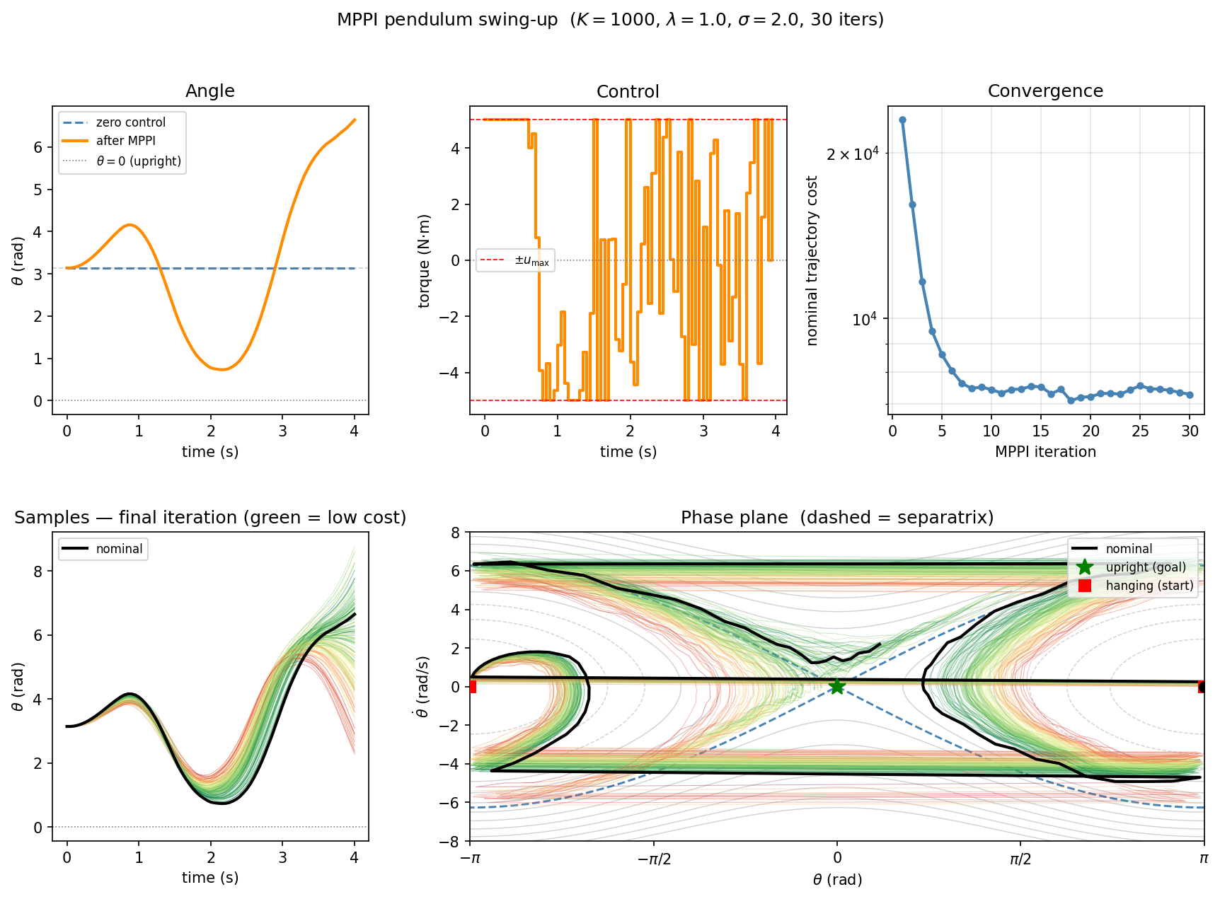
Demo

MPPI Pendulum Swing-Up

Pendulum swing-up from $\theta_0 = \pi$ (hanging down) to $\theta = 0$ or $2 \pi$ (upright).

Energy-shaping running cost: $q(x) = \bigl(E(x) - E^*\bigr)^2$, where $E(x) = \tfrac{1}{2}\dot\theta^2 + gL\cos\theta$ is the total mechanical energy and $E^* = gL$ is the energy at the upright with zero velocity.

Results

MPPI vs. iLQR / MPC

Side-by-Side Comparison

	iLQR / MPC	MPPI
Optimization	Gradient + Hessian (backward pass)	Weighted average of samples
Dynamics requirement	Differentiable $f$, Jacobians	Simulatable $f$ only
Cost requirement	Smooth, differentiable	Arbitrary (non-smooth, binary ok)
Parallelism	Sequential backward pass	Embarrassingly parallel
Global search	Local (Newton steps)	Stochastic global via samples
Stability guarantees	Lyapunov (with terminal cost)	Not guaranteed in general
Warm-starting	Natural (shift previous solution)	Natural (shift previous controls)

In practice: use iLQR/MPC when gradients are available and the landscape is well-behaved. Use MPPI for contact-rich systems, black-box simulators, or when the cost is non-differentiable.

Summary

MPPI

Core idea: replace gradient-based trajectory optimization with importance-weighted sampling.

Derivation in three steps:

1. Pose stochastic OCP as minimizing $\mathbb{E}_q[S(\tau)] + \lambda\,\mathrm{KL}(q \| p_0)$
2. Solve variationally → optimal $q^*$ is the Gibbs distribution
3. Extract control via importance sampling → no gradients needed

Key trade-offs vs. iLQR/MPC:

• + No differentiability required; handles non-smooth costs and contact
• + Massively parallelizable on GPU
• − Still needs a fast forward model
• − No convergence guarantee within one control cycle; quality scales with $K$