Optimization Theory and Practice

---

Nonlinear Least Squares

Instructor: Hasan A. Poonawala

Mechanical and Aerospace Engineering
University of Kentucky, Lexington, KY, USA

Topics:
Nonlinear Least Squares
Necessary and Sufficient Conditions
Overview of Algorithms

Forward Problems

We are often trying to work with a model that turns input $x \in \mathbb{R}^{n}$ into output $y\in \mathbb{R}^{m}$:

$$y \gets \phi_{\theta}(x),$$

where $\theta \in \mathbb{R}^p$ are the parameters of the model $\phi_{\theta}$.

Example: Given joint angles $q$, where is the robot arm’s ‘hand’? (Forward Kinematics)

Inverse Problems

The inverse problem is to find $x$ given $y$ and parameters $\theta$

$$x \gets \text{ solution of } y = \phi_{\theta}(x),$$

where $\theta \in \mathbb{R}^p$ are the parameters of the model $\phi_{\theta}$.

Example: Given where we want the robot’s arm to be, what values should we set the joint angles $q$ to? (Inverse Kinematics)

Nonlinear Least Squares

Residual (or error): $$r(x) = e(x) = y - \phi_{\theta}(x)$$ Loss: Squared Error:

$$\begin{aligned} L(x) &= e^T(x) e(x) \end{aligned}$$

$$\begin{aligned} \implies \nabla_x L(x) &= -2 e^T(x) J(x)\\ \implies \nabla_x^2 L(x) &= -2 J^T(x) J(x)- 2 \sum e_i(x) H_i(x) \end{aligned}$$

Where $J(x)$ is the Jacobian $\nabla_x \phi_{\theta}(x)$
$H_i(x)$ is the Hessian $\nabla_x^2 \phi_{\theta}(x)$

Nonlinear Least Squares

Residual (or error): $$r(x) = e(x) = y - \phi_{\theta}(x)$$ Loss: Squared Error:

$$\begin{aligned} L(x) &= e^T(x) e(x) \end{aligned}$$

$$\begin{aligned} \implies \frac{ \mathrm{ d} L(x)}{\mathrm{ d} t} &= e^T(x) \frac{ \partial e(x)}{\partial x} \dot x(t) = -e^T(x) J(x) \dot x(t) \end{aligned}$$

Choosing $\dot x(t)$ produces some $\frac{ \mathrm{ d} L(x(t))}{\mathrm{ d} t}$. What values should we want for these?

Nonlinear Least Squares

We want $\frac{ \mathrm{ d} L(x(t))}{\mathrm{ d} t} < 0$ so as to minimize $L(x(t))$ as $t \to \infty$

We can achieve that if $\frac{ \mathrm{ d} L(x)}{\mathrm{ d} t} = - e^T(x) B e(x)$

$\implies$ solve $J(x) \dot x = B e(x)$ for $\dot x$ where $B = B^T \succ 0$

Options:

1. Steepest descent: $\dot x(t) = J^T(x) e(x)$
2. Gauss-Newton direction: $\dot x(t) = J^{+} e(x)$¹
3. Levenberg–Marquardt direction: $\dot x(t) = J^{+}_{\text{damped}} e(x)$

1. $J^{+}$ is the Moore Penrose Pseudoinverse^T

Dimensions

$x \in \mathbb{R}^n$ and $\phi_{\theta}(x) \in \mathbb R^{m}$,

$\implies J(x) \in \mathbb R^(m \times n)$, $\implies e^T J(x) \in \mathbb R^(1 \times n)$

$\nabla_x L(x) \in \mathbb{R}^(1 \times n)$, $\nabla_x^{2} L(x) \in \mathbb{R}^(n \times n)$

Assume $J(x) = J$ has rank $\min(m,n)$

If $m < n$ then $J^{+} = J^T ( J J^T )_{m \times m}^{-1} \in \mathbb{R}^(n \times m)$

If $m > n$ then $J^{+} = ( J^T J )_{n \times n}^{-1} J^T \in \mathbb{R}^(n \times m)$

Compute $J^{+}$ using a singular value decomposition of $J(x)$

Aside: Supervised Machine Learning

Suppose we have data in the form of pairs $$\{x_{i},y_{i}\}_ {i \in \{1,\dots,m\}}.$$

We believe that the model is of the form $$\phi_{\theta}(x; \theta) = \theta_{1} + \theta_{2} e^{\frac{(\theta_{3}-x )^2}{\theta_{4}}} + \theta_{5} \cos(\theta_{6} x).$$

A standard approach is to find the values of $\theta_{j}$, $j \in \{1,\dots,6\}$ by solving $$\min_{\theta \in \mathbb R^6} \sum_{i=1}^{m} r_{i}^{2}(\theta)$$ where $$r_{i}(\theta) = y_{i} - \phi_{\theta}(x_i)$$

This is a nonlinear least-square problem.

However, $x_i$ are parameters and we are searching for $\theta$; opposite of previous slides

Nonlinear Least Squares

Residual (or error): $$r_{i}(\theta) = e_{i}(\theta) = y_{i} - \phi(x_{i};\theta)$$ Loss: Mean Square Error:

$$\begin{aligned} L(\theta) &= \frac{1}{m} \sum_{i=1}^{m} r_{i}^{2}(\theta) = \frac{1}{m} \sum_{i=1}^{m} r_{i}^T(\theta) r_{i}(\theta)\\ &= e^T(\theta) e(\theta)\\ \end{aligned}$$ $$\begin{aligned} \implies \nabla_\theta L(\theta) &= -2 e^T(\theta) J(\theta)\\ \implies \nabla_\theta^2 L(\theta) &= -2 J^T(\theta) J(\theta)- 2 \sum e_i(\theta) H_i(\theta) \end{aligned}$$

Where $J(\theta)$ is the Jacobian $\nabla_\theta \phi_{\theta}(x)$
$H_i(\theta)$ is the Hessian $\nabla_\theta^2 \phi_{\theta}(x_i;\theta)$

Dimensions

$\theta \in \mathbb{R}^p$ and $y_i, \phi_{\theta}(x_i;\theta),e_i \in \mathbb R$,

$\implies e \in \mathbb R^m$ $\implies J(\theta) \in \mathbb R^(m \times p)$, $\implies e^T J(\theta) \in \mathbb R^(1 \times p)$

$\nabla_\theta L(\theta) \in \mathbb{R}^(1 \times p)$, $\nabla_\theta^{2} L(\theta) \in \mathbb{R}^(p \times p)$

Assume $J(\theta) = J$ has rank $\min(m,p)$

If $m < p$ then $J^{+} = J^T ( J J^T )^{-1} \in \mathbb{R}^(p \times m)$

If $m > p$ then $J^{+} = ( J^T J )^{-1} J^T \in \mathbb{R}^(p \times m)$

Compute $J^{+}$ using a singular value decomposition of $J(\theta)$

Solutions

Global minimizer

A point $x^{*}$ is a global minimizer if $f(x^*) \leq f(x)$¹ for all $x \in \mathbb R^n$.

Local minimizer

A point $x^{*}$ is a local minimizer if there is a neighborhood $\mathcal N$ of $x^*$ where $f(x^*) \leq f(x)$ for all $x \in \mathcal N$, where a neighborhood of $y$ is an open set containing $y$.

Strict local minimizer

A point $x^{*}$ is a strict local minimizer if there is a neighborhood $\mathcal N$ of $x^*$ where $f(x^*) < f(x)$ for all $x \in \mathcal N$ with $x \neq x^*$.

1. $f(x)$ in optimizer is $L(\theta)$ in curve fitting

Summary

Condition	What we know	What it tells us	Notes
1st Ord Necessary	$x^\star$ is LM1, $f$ differentiable	$\nabla f(x^{\star})=0$	Proof justifies steepest descent
2nd Ord Necessary	$x^\star$ is LM, $f$ and $\nabla^2 f$ exist, are continuous on $\mathcal N$	$\nabla f(x^{\star})=0$ and $\nabla^2 f(x^{\star})$ is PSD
2nd Ord Sufficient	$\nabla f(x^{\star})=0$ and $\nabla^2 f(x^{\star})$ is PD	$x^\star$ is strict LM	Leads to algorithms for finding LMs
1st Ord Sufficient	$f$ is convex, $x^\star$ is LM	$x^\star$ is GM2
1st Ord Sufficient	$f$ is convex, differentiable, $\nabla f(x^{\star})=0$	$x^\star$ is GM	Leads to effective algorithms for finding global minima

1. Local Minimizer

2. Global Minimizer

Overview of Algorithms

• Recall that the algorithms are iterative
• We need a starting point $\mathbf x_0$
• … and a method to produce iterates $\mathbf{x}_1$, $\mathbf{x}_2$,$\dots$
• Generally two methods:
  • Line Search
  • Trust Region

Note

The words method and algorithm are used interchangeably

Line Search Methods

• The algorithm chooses a direction $p_k \in \mathbb{R}^n$
• Then, minimize $f(x)$ on the line defined by $\mathbf{x}_k + \alpha p_k$. That is, solve $$\min_{\alpha>0}\quad f(\mathbf{x}_k + \alpha p_k) \qquad(1)$$
  • In practice choose an $\alpha$ that makes $f(\mathbf{x}_{k+1}) < f(\mathbf{x}_{k})$, not solve Equation 1.
  • Practical method uses back-tracking line search to pick $\alpha$ given $p_k$

Line Search Methods

• Two common choices for directions.
  • Negative gradient (steepest descent) $$p_k = - \nabla f(\mathbf{x}_{k})$$
  • Newton direction: $$p_k = - (\nabla^2 f(\mathbf{x}_{k}))^{-1}\nabla f(\mathbf{x}_{k})$$

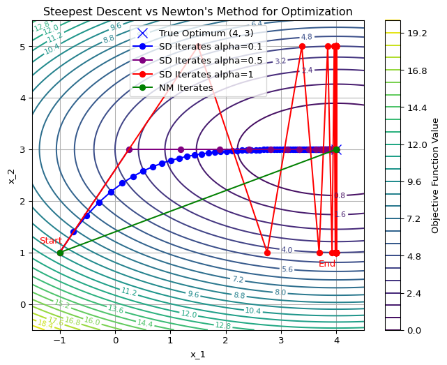
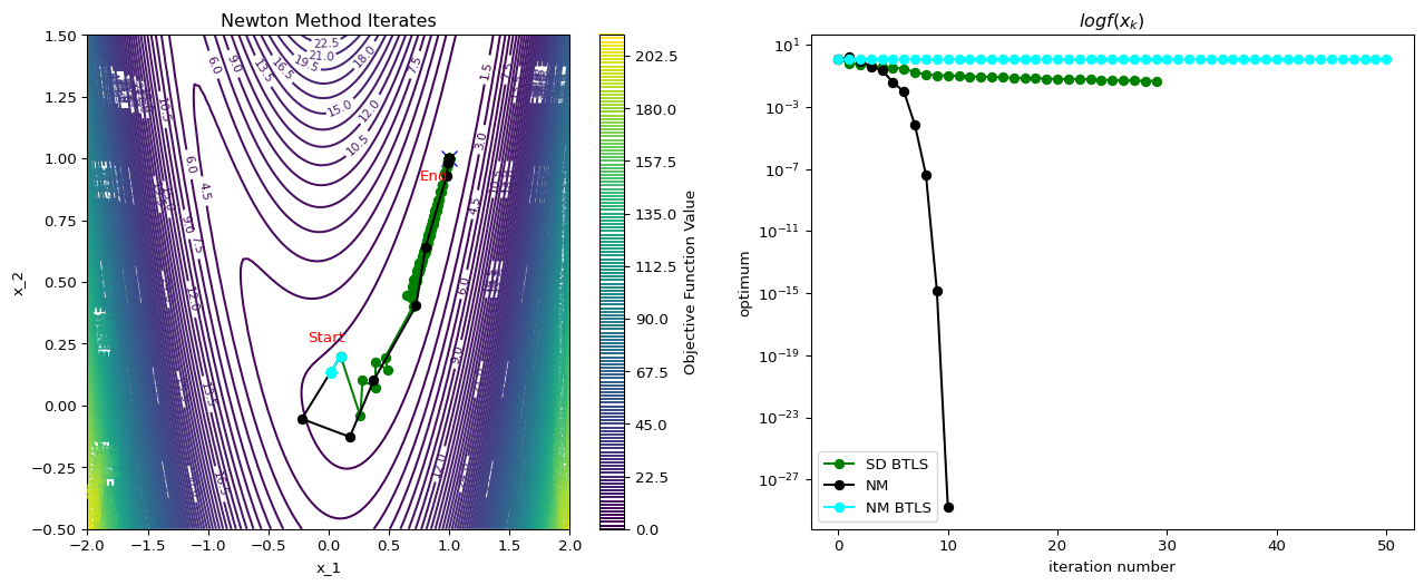
Example: Line Search Algorithms

$$\begin{align} \operatorname{minimize} & f(x) = (0.5 x_1 - 2)^2 + (x_2 - 3)^2 \end{align}$$

Important

Newton’s method is not always better

Plotting Code

import numpy as np
import matplotlib.pyplot as plt

# Define the objective function and its gradient and Hessian
def f(x, y):
    return #<answer>

def grad_f(x, y):
    """Gradient of f"""
    return np.array()

def hess_f(x, y):
    """Hessian of f"""
    return np.array()


# Steepest Descent
def steepest_descent(start, alpha=0.1,tol=1e-6, max_iter=50):
    # your code
    return x, iterates


# Plotting
x = np.linspace(-1, 4, 100)
y = np.linspace(-1, 5, 100)
X, Y = np.meshgrid(x, y)
Z = f(X, Y)

plt.figure(figsize=(8, 6))
# Contour plot of the objective function
contour = plt.contour(X, Y, Z, levels=30, cmap="viridis")
plt.clabel(contour, inline=True, fontsize=8)
plt.colorbar(contour, label="Objective Function Value")

plt.plot(4, 3, 'x', color="blue", markersize=10, label="True Optimum (4, 3)")

# Run Steepest Descent
start_point = [-1.0, 1.0]
optimum, iterates = steepest_descent(start_point)
# Extract iterate points for plotting
iterates = np.array(iterates)
x_iterates, y_iterates = iterates[:, 0], iterates[:, 1]
plt.plot(x_iterates, y_iterates, 'o-', color="blue", label="SD Iterates alpha=0.1")

# Annotate start and end points
plt.annotate("Start", (x_iterates[0], y_iterates[0]), textcoords="offset points", xytext=(-10, 10), ha="center", color="red")
plt.annotate("End", (x_iterates[-1], y_iterates[-1]), textcoords="offset points", xytext=(-10, -15), ha="center", color="red")

# Labels and legend
plt.xlabel("x_1")
plt.ylabel("x_2")
plt.title("Steepest Descent vs Newton's Method for Optimization")
plt.legend()
plt.grid(True)
plt.show()

Trust Region Methods

• Approximate $f$ near $\mathbf{x}_k$ using a model function $m_k$
• Minimize $m_k$ near $\mathbf{x}_k$ by solving $$\begin{align} \min_{p} & m_k\left(\mathbf{x}_k+p\right)\\ \text{s.t.} & \mathbf{x}_k+p \in \text{Trust region} \end{align}$$
• Common choice: local quadratic Taylor series, with a spherical trust region
  (trust-region Newton’s method)

Line Search and Trust Region Methods

In some cases, the two methods overlap ¹ $$\begin{align} \min_{p} & m_k\left(\mathbf{x}_k+p\right) = f_K + p^T \nabla f_k\\ \text{s.t.} & \| p\|_2 \leq \alpha \| \nabla f_k\|_2 \end{align}$$yields $$p = - \alpha \nabla f_{k}$$

1. $f_k = f(\mathbf{x}_k)$, $\nabla f_k = \nabla f(\mathbf{x}_k)$

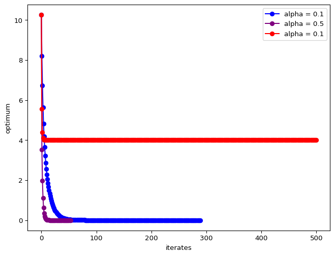
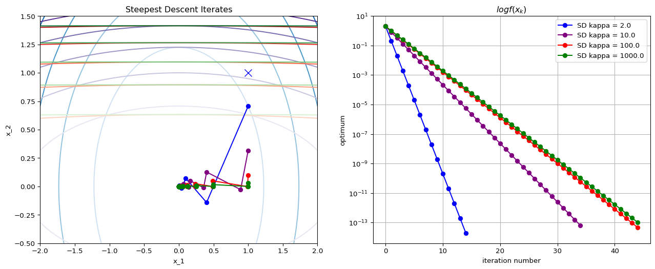
Exercise: Steepest Descent

$$\begin{align} \operatorname{minimize} & f(x) = (1 - x_1)^2 + 10 (x_2 - x_1^2)^2 \end{align}$$

The optimum is at $(1,1)$. Test the behavior of steepest descent algorithms $x_{k+1} = x_{k} - \alpha \nabla f_k$ with various constant values of $\alpha$, starting from $(0,1)$.

Solution

$$\nabla f = \begin{bmatrix} -2(1-x_1) - 40 (x_2 - x_1^2) x_1\\ 20 (x_2-x_2^2)\end{bmatrix}$$

Step size selection

Recap

• In Unconstrained Optimization we saw theory that suggests algorithms:
  • In proof of First Order Necessary Conditions, we saw that choosing $p_k = -\nabla f_k$ and $\alpha_k$ implies $f(x_{k+1}) < f(x_k)$
    • However, decreasing $f_k$ does not imply we reach the optimum if the decrease is too small
  • Another strategy from the Sufficient Conditions is to solve $\|\nabla f(x) = 0\|$
• Now we look at rules for $\alpha_k$ and $p_k$ in an algorithm $x_{k+1} = x_k + \alpha_k p_k$ that will
  • decrease $f(x_k)$ enough so that
  • we solve $\|\nabla f(x) = 0\|$

Lipschitz Function

A function $f \colon \mathbb{R}^m \to \mathbb{R}$ is Lipschitz on a set $S$ if for any $x,y \in S$ $$\|f(x) - f(y) \| \leq L \|x - y\|$$

For twice differentiable functions, $\nabla f$ being differentiable is equivalent to $$\nabla^2 f(w) \preceq L I$$ for all $w \in S$

Steepest Descent

Descent Lemma

Let $f$ be a twice differentiable function whose gradient $\nabla f$ is Lipschitz continuous over some convex set $S$. Then, for all $x,y \in S$, by Taylor’s Theorem, $$f(y) = f(x) + \nabla f(x)^T (y-x) + \frac{1}{2} (y-x)^T \nabla^2 f(z) (y-x)$$

$$\implies f(y) \leq f(x) + \nabla f(x)^T (y-x) + \frac{L}{2} \|y-x\|^2,$$

This Lemma says that we can define a local quadratic function that is an upper bound for $f$ near a point $x$.

If $x = x_k$ and $y = x_k - \alpha_k \nabla f_k$, we get $$f_{k+1} \leq f_k -\frac{\alpha_{k} (2 - L \alpha_{k} )}{2} \|\nabla f_k\|^2$$

• If $0 < \alpha_k < \frac{2}{L}$, then $f_{k+1} < f_{k}$.
• $f_{k}-f_{k+1}$ approaches zero only when $\nabla f_k \to 0$

Example

$$min_{x \in \mathbb{R}} \quad f(x) = (x-3)^2$$

$$\nabla^2 f = 2$$

To ensure decrease, we need $$\alpha < \frac{2}{L} = 1$$

If $\alpha =1$, then $f_{k+1} = f_{k}$

If $x_k = x^{\star} + y$, then $x_{k+1} = x^{\star} -y$

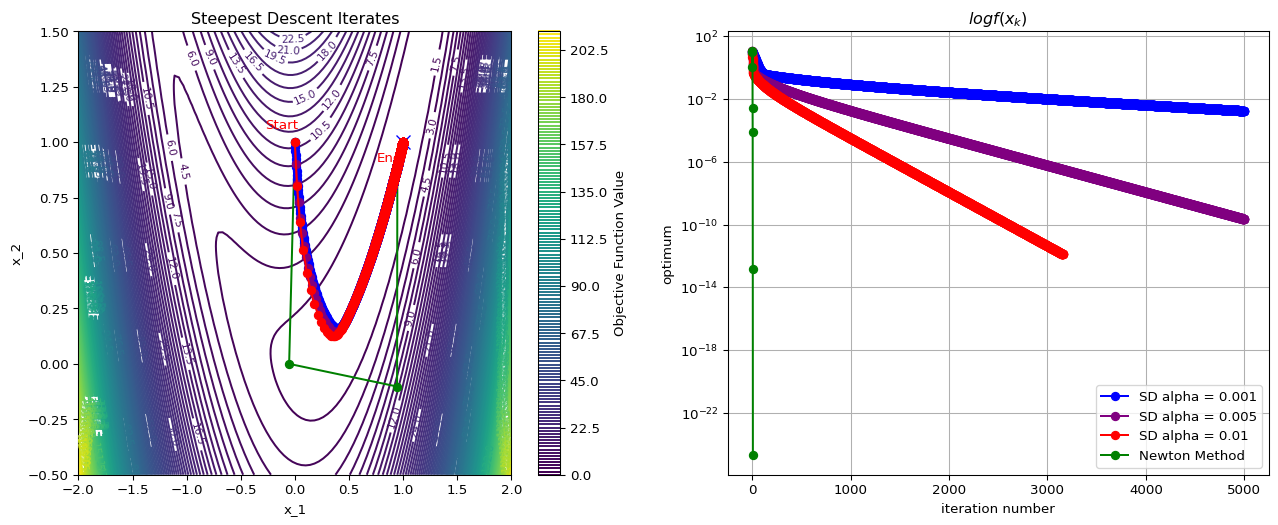
Rosenbrock Function

$$\log \epsilon = -m\ k + c \iff k = - \frac{1}{m} \log \epsilon -\frac{c}{m} \iff k = \frac{1}{m} \log \frac{1}{\epsilon} \quad + \frac{c}{m}$$

Condition Number

$$f(x,y) = x^2 + \kappa y^2$$

Newton’s Method

Motivation

• We know that whatever point we are looking must be a stationary one, it must satisfy $\nabla f(x) = 0$.

• Newton’s method applies the Newton root-finding algorithm to $\nabla f$:

  • To solve $g(x) = 0$, iteratively solve ¹ $$g(x_k) + (x_{k+1} - x_k)^T \nabla g(x) = 0 \implies x_{k+1} = x_k - (\nabla g(x) )^{\sharp} g(x)$$

• Apply root finding to $\nabla f(x) = 0$: $$x_{k+1} = x_k - (\nabla^2 f(x) )^{-1} \nabla f(x)$$

1. $\sharp$ is the left pseudo-inverse: $A^\sharp = (A^T A)^{-1} A^T$

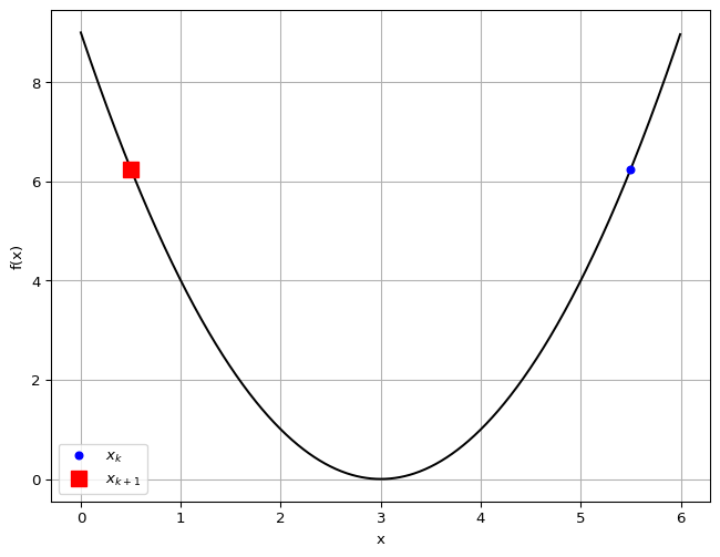
Example

• We want to find the minimizer of

$$f(x) = \frac{1}{2}x^2 - \sin{x}, \quad x_0 = \frac{1}{2}.$$

• We want an accuracy of $\varepsilon = 10^{-5}$, i.e., stop when

$$|x_{k+1} - x_k | < \varepsilon.$$

• We compute

$$f'(x) = x - \cos{x}, \quad f''(x) = 1 + \sin{x}.$$

$$\begin{align} x_1 &= \frac{1}{2} - \frac{\frac{1}{2} - \cos{\frac{1}{2}}}{1 + \sin{\frac{1}{2}}} = 0.7552, \\ x_2 &= x_1 - \frac{f'(x_1)}{f''(x_1)} = x_1 - \frac{0.02710}{1.685} = 0.7391, \\ x_3 &= x_2 - \frac{f'(x_2)}{f''(x_2)} = x_2 - \frac{9.461 \times 10^{-5}}{1.673} = 0.7390, \\ x_4 &= x_3 - \frac{f'(x_3)}{f''(x_3)} = x_3 - \frac{1.17 \times 10^{-9}}{1.673} = 0.7390. \end{align}$$

Alternate Motivation

When $\nabla^2 f_k \succ 0$, we are minimizing the quadratic approximation $$f(x) \approx f_k + \nabla f_k^T (x-x_k) + \frac{1}{2} (x-x_k)^T \nabla^2 f_k (x-x_k),$$ which need not have minimum at $x^\star$

Example: Quadratic Function

Consider $$f(x) = x^T Q x - b^T x \quad \text{ for }Q=Q^T \succ 0,$$ where $x^\star = Q^{-1} b$ $$\begin{align} \text{ Ideal update: }&& x_{k+1} &= x_k - (x_k - x^\star) = x_k - 1 \cdot (x_k - Q^{-1} b )\\ \text{Newton update:}&& x_{k+1} &= x_k + 1 \cdot (-1) \cdot Q^{-1} (Q x_k - b) = x_k -1 \cdot (x_k - Q^{-1} b)\\ \text{Steepest descent:}&& x_{k+1} &= x_k + \alpha_k \cdot (-1) \cdot (Q x_k - b) \end{align}$$

What happens when $Q = Q^T \prec 0$?

Example: Rosenbrock Function

Convergence Rate

Theorem 3.5

Suppose that $f$ is twice differentiable and that the Hessian $\nabla^2 f$ is Lipschitz continuous in a neighborhood of a solution $x^\star$ at which the sufficient conditions are satisfied. Consider the iteration $x_{k+1} = x_k + p_k$ where $p_k = - \nabla^2 f_k^{-1} \nabla f_k$. Then

• If $x_0$ is sufficiently close to $x^\star$, then $x_k \to x^\star$
• The rate of convergence $\{x_k\}$ is quadratic
• The sequence of gradient norms $\{\|\nabla f_k\|\}$ converges quadratically to zero

Newton’s Revenge

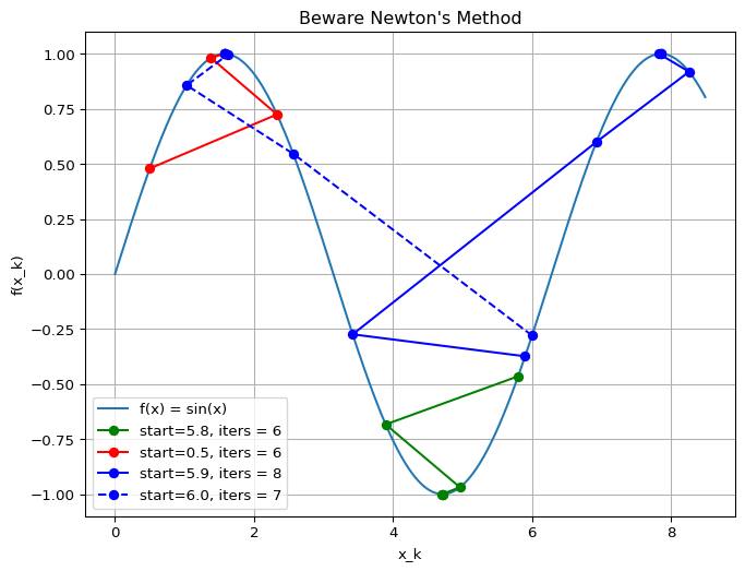
Modifications

Although Newton’s method is very attractive in terms of its convergence properties the solution, it requires modification before it can be used at points that are far from the solution.

The following modifications are typically used:

• Step-size reduction (damping)
• Modifying Hessian to be positive definite
• Approximation of Hessian

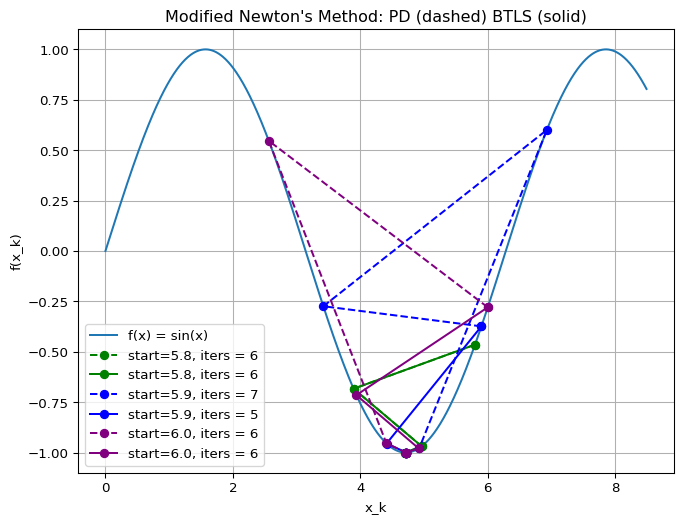
Damping

A search parameter $\alpha$ is introduced $$\bm{x}_{k+1} = \bm{x}_k - \alpha_k \nabla^2 f(\bm{x}_k)^{-1}\nabla f(\bm{x}_k),$$ where $\alpha_k$ is selected to minimize $f$.

A popular selection method is backtracking line search.

Positive Definiteness and Scaling

General class of algorithms is given by $$\bm{x}_{k+1} = \bm{x}_k + \alpha p_k = \bm{x}_k - \alpha B_k \nabla f_k, \qquad(2)$$

• SD: $B_k = \bm{I}$, Newton: $B_k = \nabla^2 f(\bm{x}_k)^{-1}$.

For small $\alpha$, it can be shown that $$f(\bm{x}_{k+1}) = f(\bm{x}_k) - \alpha \nabla f_k^T B_k \nabla f_k + O(\alpha^2).$$

• As $\alpha \rightarrow 0$, the second term on the rhs dominates the third.
• To guarantee a decrease in $f$, we must have $\nabla f_k^T B_k \nabla f_k > 0$.
  • Simplest way to ensure this is to require $B_k \succ \bm{0}$.

Positive Definiteness and Scaling

• In practice, Newton’s method must be modified to accommodate the possible non-positive definiteness of $\nabla^2 f$ at regions far from the solution.

• Common approach: $B_k = [\mu_k\bm{I} + \nabla^2 f(\bm{x}_k)]^{-1}$ for some $\mu_k > 0$.

• This can be regarded as a compromise between SD ($\mu_k$ very large) and Newton’s method ($\mu_k = 0$).

Levenberg-Marquardt performs Cholesky factorization for a given value of $\mu_k$ as follows $$\mu_k \bm{I} + \nabla^2 f(\bm{x}_k) = \bm{G}^T\bm{G}.$$

• This factorization checks implicitly for positive definiteness.

• If the factorization fails (matrix not PD) $\mu_k$ is increased.

• Step direction is found by solving $\bm{G}^T\bm{G} p_k = -\nabla f_k$.

Newton’s Revenge Avenged

Nonlinear Least Squares: Localization Example

Problem Definition

Range-Based Localization: Find position $x = (x_1, x_2)$ given noisy range measurements to known beacons.

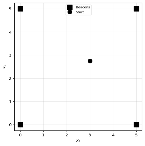
Problem Definition

Range-Based Localization: Find position $x = (x_1, x_2)$ given noisy range measurements to known beacons.

Given:

• Beacon positions $b_1, b_2, b_3, b_4 \in \mathbb{R}^2$
• Measured distances $d_1, d_2, d_3, d_4$

Residuals: $$e_i(x) = \|x - b_i\| - d_i$$

Objective: $$\min_x \sum_{i=1}^4 e_i(x)^2 = \min_x \|e(x)\|^2$$

Jacobian: Row $i$ is $$J_i = \frac{(x - b_i)^T}{\|x - b_i\|}$$

This is a unit vector pointing from beacon $i$ toward $x$.

This is a common robotics problem: GPS, UWB localization, acoustic positioning

Algorithm Comparison

Three methods to solve $\min_x \|e(x)\|^2$:

Method	Update Rule	Direction
Gradient Descent	$x_{k+1} = x_k - \alpha J^T e$	Steepest descent on $\|e\|^2$
Gauss-Newton	$x_{k+1} = x_k - (J^T J)^{-1} J^T e$	Newton with $H \approx J^T J$
Levenberg-Marquardt	$x_{k+1} = x_k - (J^T J + \lambda I)^{-1} J^T e$	Damped Gauss-Newton

Key Insights:

• GN approximates Hessian as $J^T J$, ignoring second-order residual terms $\sum e_i H_i$
• LM blends GD (large $\lambda$) and GN (small $\lambda$) via damping parameter
• Adaptive $\lambda$: increase when step rejected, decrease when accepted

Code: Localization Example

import numpy as np
import matplotlib.pyplot as plt


# Generate noisy measurements
np.random.seed(42)
noise_std = 0.1
true_distances = np.linalg.norm(beacons - true_pos, axis=1)
measured_distances = true_distances + np.random.randn(4) * noise_std

def residuals(x):
    """Compute residual vector e(x) = ||x - b_i|| - d_i"""
    return np.linalg.norm(beacons - x, axis=1) - measured_distances

def jacobian(x):
    """Compute Jacobian matrix J(x) where J_i = (x - b_i)^T / ||x - b_i||"""
    J = np.zeros((4, 2))
    for i, b in enumerate(beacons):
        diff = x - b
        norm = np.linalg.norm(diff)
        if norm > 1e-10:
            J[i] = diff / norm
    return J

def cost(x):
    """Compute sum of squared residuals"""
    e = residuals(x)
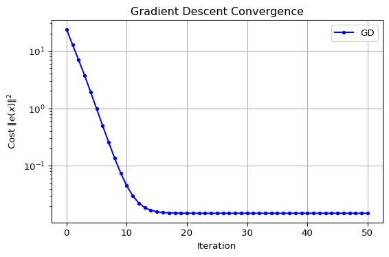
    return np.sum(e**2)

Gradient Descent for NLS

Update: $x_{k+1} = x_k - \alpha J^T e$

• Direction $-J^T e$ is gradient of $\frac{1}{2}\|e\|^2$
• Requires step size $\alpha$ selection
• Slow but reliable convergence

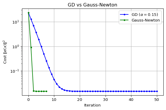
Gauss-Newton Method

Update: $x_{k+1} = x_k - (J^T J)^{-1} J^T e$

• Solves linear system $(J^T J) p = -J^T e$
• No step size needed (full step)
• Fast quadratic convergence near solution

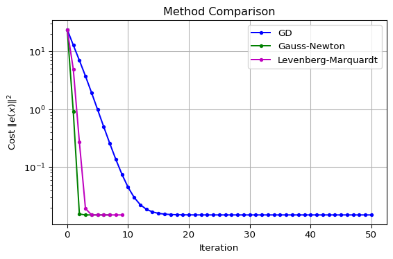
Levenberg-Marquardt Method

Update: $x_{k+1} = x_k - (J^T J + \lambda I)^{-1} J^T e$

• Adaptive $\lambda$: blend GD and GN
• Large $\lambda \to$ gradient descent (robust)
• Small $\lambda \to$ Gauss-Newton (fast)

Visualization: Iterate Paths

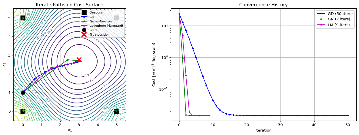
Results Discussion

Observations:

Method	Iterations	Convergence
Gradient Descent	Many (~50)	Linear rate
Gauss-Newton	Few (~5)	Quadratic near solution
Levenberg-Marquardt	Few (~5)	Adaptive, robust

Key Takeaways:

1. GD: Slow but reliable, many iterations
2. GN: Fast quadratic convergence, may fail far from solution
3. LM: Best of both worlds
   • Large $\lambda \to$ GD-like (robust)
   • Small $\lambda \to$ GN-like (fast)

When to use which?

• GD: When Jacobian is expensive or problem is poorly conditioned
• GN: Well-posed problems with good initial guess
• LM: Default choice for most NLS problems

Summary

Summary

You can now minimize $f(x)$ (when unconstrained) iteratively. Find LM $x^\star$ by

• Choosing direction $p_k$
  • Steepest descent with constant step size is easy and reliable but slow
  • Newton method is fast but expensive and unreliable
    • needs modifications for reliable convergence
  • Quasi-newton methods are a balance, but tricky
• Choosing step size $\alpha_k$
  • Back-tracking for SD and modified NM improves performance
  • Strong Wolfe conditions for Quasi-newton methods
• Not tackled: constraints, expensive $f$/$\nabla f$, discrete $x$, non-smooth $f$