The Simple Pendulum

---

A testbed for nonlinear optimal control

Instructor: Hasan A. Poonawala

Mechanical and Aerospace Engineering
University of Kentucky, Lexington, KY, USA

Topics:
Equation of motion
State space
Equilibria
Phase portrait
Swing-up goal

The Model

Equation of Motion

A torque-controlled pendulum of length $L$, mass $m$, damping $b$:

$$mL^2 \ddot\theta = mgL\sin\theta - b\dot\theta + \tau$$

Normalised (divide by $mL^2$, absorb constants into coefficients):

$$\boxed{\ddot\theta = \underbrace{1.1}_{\text{grav.}} \sin\theta \;-\; \underbrace{0.1}_{\text{damp.}}\,\dot\theta \;+\; u}$$

where $u = \tau/(mL^2)$ is the normalised torque input.

State vector: $x = \begin{bmatrix}\theta \\ \dot\theta\end{bmatrix}$

State-space form: $$\dot x = f(x, u) = \begin{bmatrix}\dot\theta \\ 1.1\sin\theta - 0.1\dot\theta + u\end{bmatrix}$$

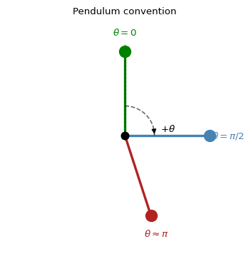
Sign Convention

$\theta$ is measured from the upright vertical

$\theta$	Position
$0$	Straight up
$\pm\pi/2$	Horizontal
$\pm\pi$	Hanging down

Positive $u$ applies torque in the direction of increasing $\theta$.

Equilibria

Where Does the Pendulum Rest?

At equilibrium: $\dot x = 0$ with $u = 0$, so $\dot\theta = 0$ and $\sin\theta = 0$.

$$\sin\theta = 0 \implies \theta = 0, \;\pm\pi, \;\pm 2\pi, \ldots$$

Two physically distinct equilibria in $[-\pi, \pi]$:

$(\theta, \dot\theta)$	Physical position	Stability
$(0,\; 0)$	Upright (balanced)	Unstable
$(\pm\pi,\; 0)$	Hanging down	Stable

Linearisation at each equilibrium — let $\theta = \theta^* + \delta\theta$:

• At $\theta^* = 0$: $\ddot{\delta\theta} \approx 1.1\,\delta\theta \;(+\text{ damping})$ → positive eigenvalue → unstable
• At $\theta^* = \pi$: $\ddot{\delta\theta} \approx -1.1\,\delta\theta \;(+\text{ damping})$ → negative eigenvalue → stable

Takeaway: without control, the pendulum settles at $\theta = \pi$ (hanging). Reaching $\theta = 0$ (upright) requires active control — even to stay there.

Phase Portrait

The Phase Plane

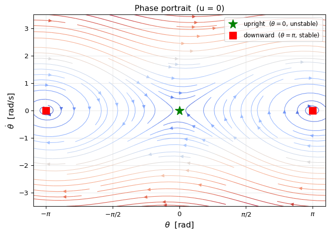
Plot $\dot\theta$ vs $\theta$ — each point is a state, arrows show $\dot x = f(x,0)$.

Reading the Phase Portrait

Closed loops around $(\pm\pi, 0)$ → oscillations near the downward equilibrium (pendulum swings back and forth without enough energy to go over the top).

Separatrix — the curves passing through $(0, 0)$ and the unstable equilibria. Trajectories inside the separatrix loop; trajectories outside spin continuously.

Damping causes the loops to spiral inward toward $(\pm\pi, 0)$ — energy is gradually lost, and the pendulum settles at rest.

The initial condition for our swing-up problem is $x_0 = (3.0,\; 0) \approx (\pi - 0.14,\; 0)$ — just to the left of the downward equilibrium.

Without Control

Zero-Control Rollout

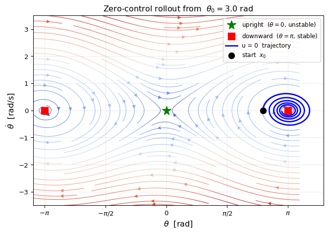
Starting at $x_0 = (3.0, 0)$ with $u \equiv 0$:

What We Observe

The trajectory spirals inward toward the downward equilibrium $(\pi, 0)$.

• Starting near $\theta = \pi$, the pendulum oscillates with decreasing amplitude
• Damping removes energy; the pendulum never reaches the upright position

The upright equilibrium $(0, 0)$ is far away in phase space — zero control cannot get us there, regardless of the initial condition (unless we start exactly there).

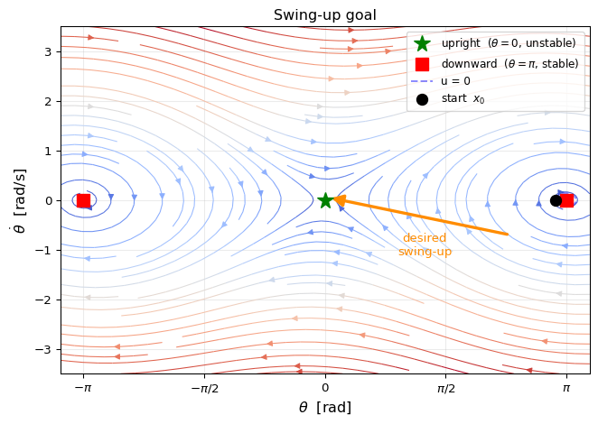
The swing-up problem: choose a control sequence $u_0, u_1, \dots, u_{T-1}$ that drives the state from $x_0 = (3.0, 0)$ to $(0, 0)$ and keeps it there.

The Swing-Up Goal

What We Want

Why is This Hard?

Nonlinearity. Linear control (e.g., LQR at the upright) only works near the goal. Starting at $\theta_0 \approx \pi$ places us far outside the linear region.

The goal is unstable. Even if we reach $(0,0)$, we must immediately switch to a stabilising controller — or include that requirement in the trajectory optimisation.

Energy must be added at the right time. The pendulum must build enough angular momentum to carry it over the top, without overshooting.

iLQR solves this by: starting from an initial (e.g., zero-control) trajectory, then iteratively refining it via local quadratic approximations of the cost and linear approximations of the dynamics — until the trajectory reaches the goal.

Summary

Concept	Value
State	$x = [\theta,\; \dot\theta]^\top$
Dynamics	$\ddot\theta = 1.1\sin\theta - 0.1\dot\theta + u$
Stable eq.	$(\pm\pi,\; 0)$ — pendulum hanging down
Unstable eq.	$(0,\; 0)$ — pendulum upright
Initial state $x_0$	$(3.0,\; 0)$ — near downward eq.
Goal	$(0,\; 0)$ — upright, balanced

The phase portrait makes clear why swing-up requires a nontrivial trajectory: the goal lies on the other side of the separatrix from the natural free motion.