def pose_to_matrix(x, y, theta):
    """Convert pose (x, y, theta) to SE(2) matrix."""
    c, s = np.cos(theta), np.sin(theta)
    return np.array([[c, -s, x], [s, c, y], [0, 0, 1]])

def matrix_to_pose(T):
    """Extract (x, y, theta) from SE(2) matrix."""
    return T[0, 2], T[1, 2], np.arctan2(T[1, 0], T[0, 0])

def compute_residual(xi, xj, z_ij):
    """
    Compute residual for edge (i, j).
    xi, xj: poses (x, y, theta)
    z_ij: measured relative pose (dx, dy, dtheta)
    Returns: residual vector [ex, ey, etheta]

    Residual: e = [R_i^T @ (p_j - p_i); theta_j - theta_i] - z_ij
    """
    x_i, y_i, theta_i = xi[0], xi[1], xi[2]
    x_j, y_j, theta_j = xj[0], xj[1], xj[2]
    dx_meas, dy_meas, dtheta_meas = z_ij[0], z_ij[1], z_ij[2]

    c, s = np.cos(theta_i), np.sin(theta_i)

    # Predicted relative position (j in frame i)
    dx_world = x_j - x_i
    dy_world = y_j - y_i
    dx_pred = c * dx_world + s * dy_world
    dy_pred = -s * dx_world + c * dy_world
    dtheta_pred = theta_j - theta_i

    # Residual = predicted - measured
    e = np.array([
        dx_pred - dx_meas,
        dy_pred - dy_meas,
        np.arctan2(np.sin(dtheta_pred - dtheta_meas),
                   np.cos(dtheta_pred - dtheta_meas))  # Wrap angle
    ])
return eDrift Visualization
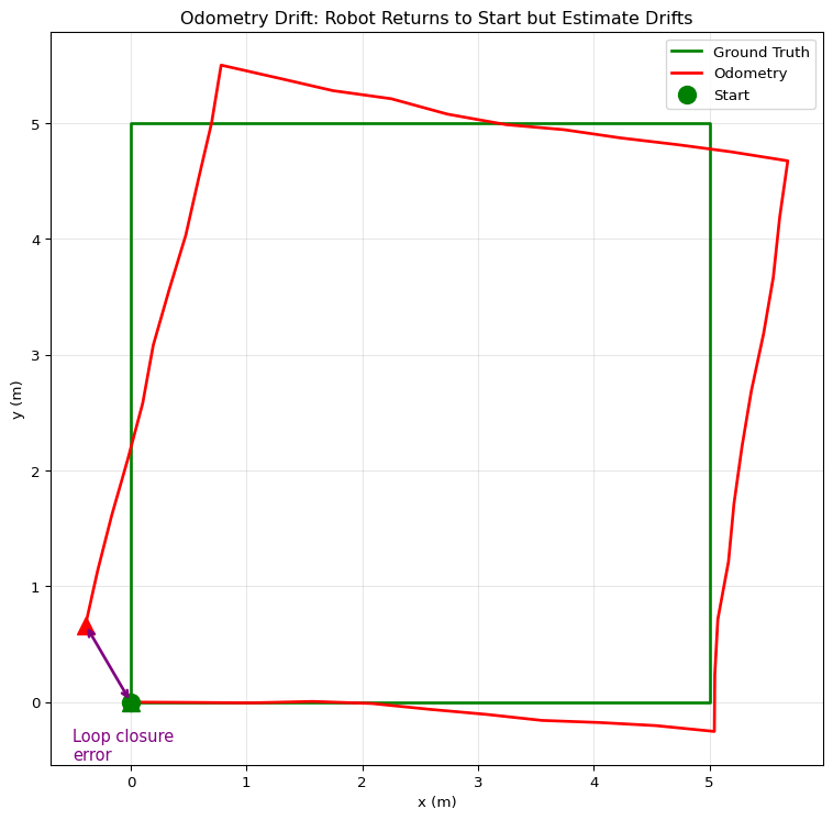
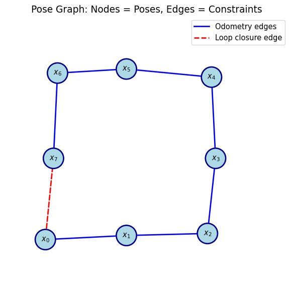
Pose Graph Representation
Sparsity Pattern
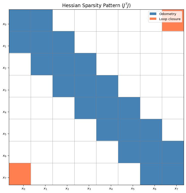
Tip
Sparsity is what makes large-scale SLAM tractable!
Example: Square Loop
Code
np.random.seed(123)

# True poses: square path
true_poses = [
    (0, 0, 0),
    (2, 0, 0),
    (4, 0, np.pi/2),
    (4, 2, np.pi/2),
    (4, 4, np.pi),
    (2, 4, np.pi),
    (0, 4, -np.pi/2),
    (0, 2, -np.pi/2),
]

# Generate noisy odometry measurements
edges = [(i, i+1) for i in range(7)]  # Sequential
edges.append((7, 0))  # Loop closure!

measurements = []
for i, j in edges:
    Ti = pose_to_matrix(*true_poses[i])
    Tj = pose_to_matrix(*true_poses[j])
    T_rel = np.linalg.inv(Ti) @ Tj
    z = matrix_to_pose(T_rel)
    # Add noise (more noise on odometry, less on loop closure)
    if j == i + 1:  # Odometry
        noise = np.array([0.1, 0.1, 0.05]) * np.random.randn(3)
    else:  # Loop closure (often more accurate)
        noise = np.array([0.05, 0.05, 0.02]) * np.random.randn(3)
    measurements.append(tuple(np.array(z) + noise))

# Initial poses from chaining odometry (with drift)
initial_poses = [np.array([0.0, 0.0, 0.0])]
T_acc = np.eye(3)
for i in range(7):
    T_rel = pose_to_matrix(*measurements[i])
    T_acc = T_acc @ T_rel
    initial_poses.append(np.array(matrix_to_pose(T_acc)))

# Optimize
optimized_poses = optimize_pose_graph(initial_poses, edges, measurements, n_iter=20)

# Plot comparison
fig, axes = plt.subplots(1, 2, figsize=(12, 5))

# Before optimization
ax = axes[0]
init_arr = np.array(initial_poses)
true_arr = np.array(true_poses)
ax.plot(true_arr[:, 0], true_arr[:, 1], 'g-o', markersize=8, linewidth=2, label='Ground Truth')
ax.plot(init_arr[:, 0], init_arr[:, 1], 'r-s', markersize=8, linewidth=2, label='Initial (Odometry)')
# Draw loop closure gap
ax.plot([init_arr[-1, 0], init_arr[0, 0]], [init_arr[-1, 1], init_arr[0, 1]],
        'r--', linewidth=2, alpha=0.5)
ax.set_xlabel('x (m)')
ax.set_ylabel('y (m)')
ax.set_aspect('equal')
ax.grid(True, alpha=0.3)
ax.legend()
ax.set_title('Before Optimization')

# After optimization
ax = axes[1]
opt_arr = np.array(optimized_poses)
ax.plot(true_arr[:, 0], true_arr[:, 1], 'g-o', markersize=8, linewidth=2, label='Ground Truth')
ax.plot(opt_arr[:, 0], opt_arr[:, 1], 'b-s', markersize=8, linewidth=2, label='Optimized')
ax.set_xlabel('x (m)')
ax.set_ylabel('y (m)')
ax.set_aspect('equal')
ax.grid(True, alpha=0.3)
ax.legend()
ax.set_title('After Optimization')

plt.tight_layout()
plt.show()

# Print errors
init_error = np.mean([np.linalg.norm(init_arr[i, :2] - true_arr[i, :2]) for i in range(8)])
opt_error = np.mean([np.linalg.norm(opt_arr[i, :2] - true_arr[i, :2]) for i in range(8)])
print(f"Mean position error - Initial: {init_error:.3f} m, Optimized: {opt_error:.3f} m")
Mean position error - Initial: 0.593 m, Optimized: 0.152 m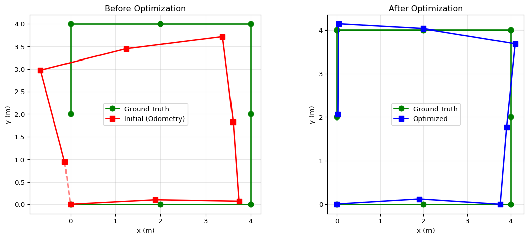
Convergence
Code
# Track cost over iterations
def compute_total_cost(poses, edges, measurements):
    cost = 0
    for (i, j), z_ij in zip(edges, measurements):
        e = compute_residual(poses[i], poses[j], z_ij)
        cost += e @ e
    return cost

# Re-run optimization tracking cost
poses = [np.array(p) for p in initial_poses]
costs = [compute_total_cost(poses, edges, measurements)]

for iteration in range(20):
    H, b = build_linear_system(poses, edges, measurements)
    H[0:3, 0:3] += 1e6 * np.eye(3)
    dx = np.linalg.solve(H, -b)
    for i in range(len(poses)):
        poses[i] = poses[i] + dx[3*i:3*i+3]
        poses[i][2] = np.arctan2(np.sin(poses[i][2]), np.cos(poses[i][2]))
    costs.append(compute_total_cost(poses, edges, measurements))

fig, ax = plt.subplots(figsize=(8, 5))
ax.semilogy(costs, 'b-o', markersize=6)
ax.set_xlabel('Iteration')
ax.set_ylabel('Cost (log scale)')
ax.set_title('Gauss-Newton Convergence')
ax.grid(True, alpha=0.3)
plt.tight_layout()
plt.show()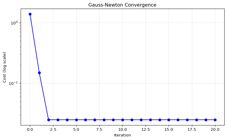
Note
Gauss-Newton converges quickly — typically 5-10 iterations suffice.
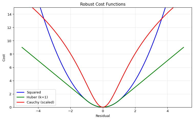
Robust Cost Visualization
Factor Graph View
GTSAM uses “factor graph” terminology:
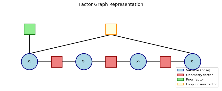
Note
Variables are poses, factors are constraints (measurements). Same math, different visualization!