Proximal Policy Optimization

---

PPO: Model-Free Reinforcement Learning

Instructor: Hasan A. Poonawala

Mechanical and Aerospace Engineering
University of Kentucky, Lexington, KY, USA

Topics:
Bridge from MPPI
Policy gradient theorem
Importance sampling & trust regions
Clipped surrogate objective
Advantage estimation
Algorithm and properties

A Progression in Optimal Control

Each method relaxes one key assumption of the previous.

Method	Dynamics	Key relaxation
LQR	linear	baseline: analytical solution
iLQR	nonlinear	drop linearity via local linearization
MPC	nonlinear	drop infinite horizon; add constraints; replan online
MPPI	nonlinear	drop differentiability; use sampling
PPO	unknown	drop the model entirely; learn from interaction

Every method above requires a access to a dynamics model $f$. PPO removes that requirement.

From MPPI to PPO

MPPI

MPPI moves through these distributions in each planning step:

$$\underbrace{\varepsilon \sim \mathcal{N}(0,\Sigma)}_{\text{1. noise dist}} \;\longrightarrow\; \underbrace{u_t = v_t + \varepsilon_t}_{\text{2. control dist}} \;\longrightarrow\; \underbrace{\tau \text{ via } x_{t+1}=f(x_t,u_t)}_{\text{3. trajectory dist}} \;\longrightarrow\; \underbrace{S(\tau)}_{\text{4. Cost distribution}}$$

The parameter being optimized is $v_t$ — the mean of the control distribution — a fixed sequence of vectors.

The update is a cost-weighted mean: $$v_t \leftarrow v_t + \sum_k \tilde{w}^{(k)} \varepsilon_t^{(k)}, \qquad \tilde{w}^{(k)} \propto \exp\!\left(-S^{(k)}/\lambda\right)$$

The optimized object $v_t$ is an open-loop control sequence: it does not depend on state encountered during execution.

PPO

PPO inserts an additional level — a parameterized state-dependent policy:

$$\underbrace{\theta}_{\text{1. param space}} \;\longrightarrow\; \underbrace{\pi_\theta(a \mid s)}_{\text{2. action dist (per state)}} \;\longrightarrow\; \underbrace{a_t \sim \pi_\theta(\cdot \mid s_t)}_{\text{3. trajectory dist}} \;\longrightarrow\; \underbrace{R(\tau)}_{\text{4. Reward distribution}}$$

The parameter being optimized is $\theta$ — the weights of a neural network (or other function approximator) that maps any state to a distribution over actions.

The update adjusts $\theta$ so that actions leading to higher reward become more probable.

	MPPI	PPO
Optimized object	control sequence $v_{0:T-1}$	policy params $\theta$
Action at runtime	fixed per step	$a \sim \pi_\theta(\cdot \mid s)$
Feedback	open-loop (replanned each cycle)	closed-loop (state-dependent)
Dynamics model	required	not required

The Bridge: Same Core Mechanism

Despite the structural difference, MPPI and PPO share the same core update principle:

Sample trajectories under the current distribution.

Weight samples by reward (or advantage).

Update the parameter toward the higher-weight samples.

The proximal constraint in PPO plays the same role as the KL penalty in MPPI’s information-theoretic derivation: both prevent the update from stepping so far from the current distribution that the importance weights become unreliable.

MPPI	PPO
$\min_q\;\mathbb{E}_q[S] + \lambda\,\mathrm{KL}(q \| p_0)$	$\max_\theta\;\mathbb{E}[\text{clipped IS ratio} \times A]$1
KL term limits policy change	clipping limits policy change

1. IS: Importance Sampling; A: Advantage

Policy Gradient Setup

The Reinforcement Learning Objective

An agent interacts with an environment: at each step $t$ it observes state $s_t$, takes action $a_t \sim \pi_\theta(\cdot \mid s_t)$, and receives reward $r_t$.

Goal: find $\theta$ to maximize expected discounted return:

$$J(\theta) = \mathbb{E}_{\tau \sim \pi_\theta}\!\left[\sum_{t=0}^{T} \gamma^t r_t\right]$$

where $\gamma \in (0,1]$ is a discount factor and $\tau = (s_0, a_0, r_0, s_1, a_1, r_1, \ldots)$.

Unlike MPPI, no dynamics model $f$ appears. The reward signal arrives directly from the environment. The only requirement is that $\pi_\theta(a \mid s)$ is differentiable in $\theta$.

Reinforcement Learning uses an estimated value function $V(s)$ or $Q$-Value $Q(s,a)$ to summarize what will happen, instead of an explicit model $f$.

Value Functions and Advantage

Define:

$$V^\pi(s) = \mathbb{E}_{\tau \sim \pi}\!\left[\sum_{t'=t}^T \gamma^{t'-t} r_{t'} \;\Big|\; s_t = s\right]$$

the state-value function — expected return from state $s$ under policy $\pi$.

$$Q^\pi(s,a) = \mathbb{E}_{\tau \sim \pi}\!\left[\sum_{t'=t}^T \gamma^{t'-t} r_{t'} \;\Big|\; s_t = s,\; a_t = a\right]$$

the action-value function — expected return after taking action $a$ in state $s$.

$$A^\pi(s,a) = Q^\pi(s,a) - V^\pi(s)$$

the advantage — how much better (or worse) action $a$ is than the average action from state $s$.

$A > 0$: this action is better than average — make it more probable. $A < 0$: worse than average — make it less probable.

Advantages as shortcuts

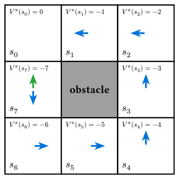
$r(s) = -1$ for all states except $s_0$.

So, under blue policy, $V(s_i) = - i$

$Q(s_7,\text{"up"}) = -1$

$$\begin{align} \implies A^{\pi}(s_7, \text{"up"}) &= Q(s_7,\text{"up"}) - V(s_7)\\ &= -1 - (-7) \\&= 6 \end{align}$$

Stochastic Policy

A simple and commonly used stochastic state-dependent policy is Gaussian:

$\pi_\theta(a | s) = \frac{1}{\sqrt{2 \pi } \sigma} \exp^{ - \left(\frac{a - \mu_\theta(s)}{ \sigma} \right)^2}$

• $\mu_\theta(s)$ is a state-dependent ‘mean action’.
  Example: at $x=1$ meters average force is $-1$ N to push a box back to $x=0$
• $\sigma$ is independent of $\theta$ and $s$ to simplify computations

Policy Gradient Theorem

The gradient of $J(\theta)$ with respect to $\theta$ is:

$$\nabla_\theta J(\theta) = \mathbb{E}_{\tau \sim \pi_\theta}\!\left[\sum_t \nabla_\theta \log \pi_\theta(a_t \mid s_t) \cdot R(\tau)\right]$$

This is the policy gradient theorem (PGT). Key observations:

• Only $\log \pi_\theta$ needs to be differentiable — the environment dynamics need not be.
• $\nabla_\theta \log \pi_\theta(a \mid s)$: direction in $\theta$-space that increases the probability of $a$ at $s$.
  • $\pi_\theta(a | s) = \frac{1}{\sqrt{2 \pi } \sigma} \exp^{ - \left(\frac{a - \mu_\theta(s)}{ \sigma} \right)^2} \implies \nabla_\theta \log \pi_\theta(a | s) = (a - \mu_\theta(s) ) \nabla_\theta \mu_\theta(s)$
  • Brings $\mu_\theta(s)$ closer to $a$, increasing probability of action $a$
• Multiplied by $R(\tau)$: More rewards imply greater increase in probability of that action relative to others

Algorithms using PGT

REINFORCE: Simulate using stochastic actions, implement PGT as-is using actual rewards $$\nabla_\theta J(\theta) = \mathbb{E}_{\tau \sim \pi_\theta}\!\left[\sum_t \nabla_\theta \log \pi_\theta(a_t \mid s_t) \cdot R(\tau)\right]$$

Vanilla policy gradient: Remove a baseline $b(s)$ from actual rewards. Usually $b(s) = V^{\pi}(s)$. $$\nabla_\theta J(\theta) = \mathbb{E}_{\tau \sim \pi_\theta}\!\left[\sum_t \nabla_\theta \log \pi_\theta(a_t \mid s_t) \cdot ( R(\tau) - b(s_t) )\right]$$ Why: reduces variance without introducing any bias

Actor-Critic: Use a critic function to estimate $R(\tau)$, not actual rewards. A popular critic is the advantage function.

$$\theta \leftarrow \theta + \alpha \sum_t \nabla_\theta \log \pi_\theta(a_t \mid s_t) \cdot \hat{A}_t$$

Probability of better actions ($A_t>0$) increases while that of worse actions ($A_t <0$) decreases

Why Actor-Critic Is Unstable

Actor-Critic methods work in principle but fails in practice due to step-size sensitivity:

• Too small a step → slow convergence, wasted samples
• Too large a step → the policy changes drastically, old samples are no longer representative, and the update may push into a region from which recovery is difficult

The fundamental issue: gradient ascent in $\theta$-space does not respect the geometry of the probability distribution $\pi_\theta$. A small step in $\theta$ can produce a large change in $\pi_\theta$.

TRPO (Trust Region Policy Optimization) solved this by constraining $\mathrm{KL}(\pi_{\theta_\mathrm{old}} \| \pi_\theta) \leq \delta$, but it requires second-order optimization (conjugate gradient + line search) — expensive.

PPO achieves similar stability with a simple first-order trick: clip the importance ratio.

The PPO Objective

Importance Sampling Enters

Suppose we collected data under $\pi_{\theta_\mathrm{old}}$. We want to optimize $\theta$ using those samples — this is importance sampling.

Define the probability ratio:

$$r_t(\theta) = \frac{\pi_\theta(a_t \mid s_t)}{\pi_{\theta_\mathrm{old}}(a_t \mid s_t)}$$

Then the policy gradient objective can be written as:

$$L^\mathrm{IS}(\theta) = \mathbb{E}_t\!\left[r_t(\theta)\, A_t\right]$$

This is exactly the importance-sampling reweighting from MPPI: we collected samples under $\pi_{\theta_\mathrm{old}}$ (analogous to $p_0$), and reweight by $r_t(\theta)$ (analogous to $\exp(-S/\lambda)$) to estimate expectations under the new distribution.

Problem: $A_t$ comes from $\theta_{\mathrm{old}}$. Unconstrained maximization of $L^\mathrm{IS}$ can push $r_t$ to extreme values. If $\pi_\theta$ moves far from $\pi_{\theta_\mathrm{old}}$ ($r_t$ far from $1$), the associated gradient is unreliable and the update collapses.

The Clipped Surrogate Objective

PPO replaces $L^\mathrm{IS}$ with a clipped version:

$$L^\mathrm{CLIP}(\theta) = \mathbb{E}_t\!\left[\min\!\left(r_t(\theta)\,A_t,\;\mathrm{clip}(r_t(\theta),\,1-\varepsilon,\,1+\varepsilon)\,A_t\right)\right]$$

where $\varepsilon \approx 0.2$ is a small hyperparameter.

Intuition for the clip:

When $|r_t(\theta) - 1| > \epsilon$, the gradient of the clipped term w.r.t $\theta$ is zero, no update when the probabilities have changed too much going from $\theta_{old} \to \theta$.

Intuition for the min:

Makes the clipping asymmetric: only clip when

• $A_t > 0$ and new probability under $\theta$ is already much higher at current $\theta$
• $A_t < 0$ and new probability under $\theta$ is already much lower at current $\theta$

Clipping prevents the policy from taking greedy steps that move it outside the region where the current samples are informative — the same motivation as the KL term in MPPI.

Advantage Estimation

Estimating $A_t$ in Practice

The true advantage $A_t = Q^\pi(s_t,a_t) - V^\pi(s_t)$ is unknown. Two practical estimators:

Monte Carlo return: $$\hat{A}_t^\mathrm{MC} = \left(\sum_{t'=t}^T \gamma^{t'-t} r_{t'}\right) - V_\phi(s_t)$$

Unbiased but high variance — a single sampled return can be far from the mean.

TD residual (1-step): $$\hat{A}_t^\mathrm{TD} = r_t + \gamma V_\phi(s_{t+1}) - V_\phi(s_t)$$

Low variance but biased if $V_\phi$ is inaccurate.

Generalized Advantage Estimation (GAE): interpolate with parameter $\hat\lambda \in [0,1]$: $$\hat{A}_t^\mathrm{GAE} = \sum_{k=0}^{T-t} (\gamma\hat\lambda)^k \delta_{t+k}, \qquad \delta_t = r_t + \gamma V_\phi(s_{t+1}) - V_\phi(s_t)$$

$\hat\lambda = 0$: pure TD (low variance, more bias); $\hat\lambda = 1$: Monte Carlo (unbiased, high variance).

The Critic: Learning $V_\phi$

PPO jointly trains two networks (or one with two heads):

Actor $\pi_\theta(a \mid s)$: the policy — updated via $L^\mathrm{CLIP}$.

Critic $V_\phi(s)$: the value function — updated by minimizing the TD error: $$L^\mathrm{VF}(\phi) = \mathbb{E}_t\!\left[\left(V_\phi(s_t) - \hat{V}_t^\mathrm{target}\right)^2\right]$$

The full PPO loss also includes an entropy bonus to encourage exploration:

$$L^\mathrm{PPO}(\theta,\phi) = L^\mathrm{CLIP}(\theta) - c_1 L^\mathrm{VF}(\phi) + c_2\, \mathbb{E}_t[\mathcal{H}(\pi_\theta(\cdot \mid s_t))]$$

There is no equivalent of the critic in MPPI — MPPI uses the raw trajectory cost $S(\tau)$ directly rather than learning a value function from data.

The Algorithm

PPO

Input: policy π_θ, value network V_φ, clip ε, rollout length T, epochs K

Repeat until convergence:
  1. Collect rollout:
       For t = 0 to T-1:
         a_t ~ π_θ(· | s_t),  step environment,  observe r_t, s_{t+1}

  2. Compute advantages and target values:
       δ_t  = r_t + γ V_φ(s_{t+1}) − V_φ(s_t)
       Â_t  = GAE(δ_0:T, λ̂)      (generalized advantage estimate)
       V̂_t  = Â_t + V_φ(s_t)     (target for critic)

  3. Save old policy:  θ_old ← θ

  4. Optimize for K epochs over the collected batch:
       For each minibatch (s_t, a_t, Â_t, V̂_t):
         r_t(θ) = π_θ(a_t | s_t) / π_{θ_old}(a_t | s_t)
         L^CLIP  = mean[ min( r_t Â_t,  clip(r_t, 1−ε, 1+ε) Â_t ) ]
         L^VF    = mean[ (V_φ(s_t) − V̂_t)² ]
         L^H     = mean[ H(π_θ(· | s_t)) ]   (entropy bonus)
         Update θ, φ by gradient ascent on  L^CLIP − c₁ L^VF + c₂ L^H

  5. Repeat from step 1.

Steps 1–2 collect experience; step 4 reuses it for multiple gradient updates (multiple epochs over the same batch), which is more sample-efficient than one-step REINFORCE. The clip makes multi-epoch reuse safe.

What PPO Gives You

Property	Explanation
Model-free	No dynamics model needed; learns purely from $(s,a,r,s')$ tuples
Closed-loop	Policy $\pi_\theta(a \mid s)$ adapts to any visited state
Stable updates	Clipping prevents destructive large steps; robust to learning rate
Sample reuse	Multiple gradient epochs per rollout batch
Continuous or discrete actions	Gaussian policy for continuous; softmax for discrete
GPU-friendly	Parallel environment rollouts; batch backprop through the network

What PPO still requires: enough environment interactions to learn a good value function and policy. Sample efficiency is better than REINFORCE but far lower than model-based methods like MPPI. PPO may need millions of environment steps for complex tasks.

Hyperparameters

Parameter	Effect	Typical value
$\varepsilon$ (clip range)	Larger → more aggressive update	0.1–0.3
$T$ (rollout length)	Longer → better return estimates	128–4096 steps
$K$ (update epochs)	More → better use of each batch	3–10
$\hat\lambda$ (GAE)	Bias-variance tradeoff in advantage	0.95
$\gamma$ (discount)	Effective planning horizon $\approx 1/(1-\gamma)$	0.99
$c_1, c_2$ (loss weights)	Value vs. entropy tradeoff	$c_1=0.5$, $c_2=0.01$

PPO is often described as the “default” deep RL algorithm because its performance is robust across a wide range of hyperparameter settings — the clip replaces careful learning-rate tuning.

MPPI vs. PPO

	MPPI	PPO
Dynamics model	Required (must simulate $f$)	Not required
Control structure	Open-loop sequence $v_{0:T-1}$	Closed-loop policy $\pi_\theta(a \mid s)$
Distribution chain	noise → control → trajectory → cost	$\theta$ → policy → action → trajectory → reward
Optimization object	Control mean $v_t$	Policy params $\theta$
“Proximity” mechanism	KL penalty $\lambda\,\mathrm{KL}(q \| p_0)$	Ratio clip $\mathrm{clip}(r_t, 1\pm\varepsilon)$
Sample efficiency	High (model-based)	Lower (model-free)

RL Algorithm Landscape

Taxonomy of Key Algorithms

Algorithm	Policy	On/Off-policy	Action space	Needs critic	Key mechanism
REINFORCE	stochastic	on	discrete / cont.	no	Monte Carlo returns
A2C / A3C	stochastic	on	discrete / cont.	yes ($V$)	parallel workers + TD advantage
PPO	stochastic	on	discrete / cont.	yes ($V$)	clipped IS ratio; multi-epoch reuse
TD3	deterministic	off	continuous	yes (twin $Q$)	fixes DDPG overestimation
SAC	stochastic	off	continuous†	yes (twin $Q$)	entropy regularization; max-entropy framework

†Discrete SAC exists but is less common.

On-policy algorithms discard data after each update — samples must come from the current policy. Off-policy algorithms store data in a replay buffer and can reuse old transitions, making them more sample-efficient but harder to stabilize.

Choosing an Algorithm

Action space drives the first cut:

• Discrete actions (game buttons, token selection): REINFORCE, A2C, PPO
• Continuous actions (joint torques, velocities): PPO, TD3, SAC, DDPG

Sample budget drives the second cut:

• Data is cheap (fast simulator, parallelizable): on-policy methods (PPO, ACKTR) are simpler and competitive
• Data is expensive (real hardware, slow sim): off-policy methods (SAC, TD3) extract more from each transition