Scan Matching

---

ICP and NDT

Instructor: Hasan A. Poonawala

Mechanical and Aerospace Engineering
University of Kentucky, Lexington, KY, USA

Topics:
2D Rigid Transformations
ICP Algorithm
Point Cloud Alignment

Lesson Overview

1. Mathematical Foundations: 2D rigid transformations and SE(2)
2. Algorithm Walkthrough: Iterative Closest Point (ICP)
3. Practical Intuition: Convergence, local minima, debugging
4. Assignment: Scan matching for pose estimation and SLAM

Connection: This applies nonlinear least squares to a real robotics problem

Background: LiDAR Sensors

2D LiDAR Sensor

• Rotating mirror/sensor emits laser pulses
• Scans across a horizontal or vertical plane
• Returns points in polar coordinates $(r_i, \phi_i)$
• Corresponds to nearest reflective object along direction $\phi_i$

A relatively inexpensive 2D LiDAR

2D LiDAR Sensor

Depiction of LiDAR scan

LiDAR Data Format

Points returned in polar coordinates $(r_i, \phi_i)$

Converted to Cartesian coordinates: $$\begin{aligned} x_i &= r_i \cos \phi_i \\ y_i &= r_i \sin \phi_i \end{aligned}$$

Note

Data provided in Cartesian coordinates with units in meters

Scan Matching: Core Idea

When a robot moves, the LiDAR captures distances from different positions

Key insight: If motion is small, we can estimate it by aligning consecutive scans

• Points corresponding to the same physical object should overlap
• “Walls” in nearby scans should lie on top of each other

Scan Matching: Visualization

Before alignment

Two scans in their respective robot frames

After alignment

Correctly transformed scans overlap

Scan matching - unaligned (left) vs aligned (right)

Part 1: Mathematical Foundations

2D Rotation Matrix

A rotation by angle $\theta$ in 2D is represented by:

$$R(\theta) = \begin{bmatrix} \cos\theta & -\sin\theta \\ \sin\theta & \cos\theta \end{bmatrix}$$

Properties:

• $R(\theta)^T = R(-\theta) = R(\theta)^{-1}$ (orthogonal)
• $\det(R(\theta)) = 1$ (preserves orientation)
• $R(\theta_1) R(\theta_2) = R(\theta_1 + \theta_2)$ (composition)

Rotation Derivation

How does $R(\theta)$ arise? Consider rotating point $(x, y)$:

Original point in polar form: $$\begin{aligned} x &= r\cos\alpha \\ y &= r\sin\alpha \end{aligned}$$

After rotation by $\theta$: $$\begin{aligned} x' &= r\cos(\alpha + \theta) \\ y' &= r\sin(\alpha + \theta) \end{aligned}$$

Expanding using angle addition formulas: $$\begin{aligned} x' &= r\cos\alpha\cos\theta - r\sin\alpha\sin\theta = x\cos\theta - y\sin\theta \\ y' &= r\cos\alpha\sin\theta + r\sin\alpha\cos\theta = x\sin\theta + y\cos\theta \end{aligned}$$

Visualizing 2D Rotation

import numpy as np
import matplotlib.pyplot as plt

def rotation_matrix(theta):
    """2D rotation matrix for angle theta (radians)."""
    c, s = np.cos(theta), np.sin(theta)
    return np.array([[c, -s], [s, c]])

# Create a simple shape (house)
house = np.array([[0, 1, 1, 0.5, 0, 0], [0, 0, 1, 1.5, 1, 0]])

fig, axes = plt.subplots(1, 3, figsize=(10, 3))
angles = [0, np.pi/4, np.pi/2]
titles = [r'$\theta = 0$', r'$\theta = \pi/4$', r'$\theta = \pi/2$']

for ax, theta, title in zip(axes, angles, titles):
    R = rotation_matrix(theta)
    rotated = R @ house
    ax.plot(house[0], house[1], 'b--', alpha=0.5, label='Original')
    ax.fill(house[0], house[1], alpha=0.2)
    ax.plot(rotated[0], rotated[1], 'r-', linewidth=2, label='Rotated')
    ax.fill(rotated[0], rotated[1], alpha=0.3, color='red')
    ax.set_xlim(-2, 2); ax.set_ylim(-1, 2.5)
    ax.set_aspect('equal'); ax.grid(True, alpha=0.3)
    ax.set_title(title); ax.legend(fontsize=8)

plt.tight_layout()
plt.show()

 

2D Rigid Transformation

A rigid transformation combines rotation and translation:

$$\mathbf{p}' = R(\theta)\mathbf{p} + \mathbf{t}$$

where $\mathbf{p} = \begin{bmatrix} x \\ y \end{bmatrix}$ and $\mathbf{t} = \begin{bmatrix} t_x \\ t_y \end{bmatrix}$

Expanded form: $$\begin{bmatrix} x' \\ y' \end{bmatrix} = \begin{bmatrix} \cos\theta & -\sin\theta \\ \sin\theta & \cos\theta \end{bmatrix} \begin{bmatrix} x \\ y \end{bmatrix} + \begin{bmatrix} t_x \\ t_y \end{bmatrix}$$

Homogeneous Coordinates

To compose transformations easily, use homogeneous coordinates:

$$\begin{bmatrix} x' \\ y' \\ 1 \end{bmatrix} = \begin{bmatrix} \cos\theta & -\sin\theta & t_x \\ \sin\theta & \cos\theta & t_y \\ 0 & 0 & 1 \end{bmatrix} \begin{bmatrix} x \\ y \\ 1 \end{bmatrix}$$

This $3 \times 3$ matrix is an element of SE(2) — the Special Euclidean group in 2D

SE(2): The Group of 2D Rigid Motions

$$T = \begin{bmatrix} R & \mathbf{t} \\ \mathbf{0} & 1 \end{bmatrix} \in SE(2)$$

Why a group?

• Closure: $T_1 T_2 \in SE(2)$ (composing motions gives a motion)
• Identity: $I_{3\times 3}$ (no motion)
• Inverse: $T^{-1} = \begin{bmatrix} R^T & -R^T\mathbf{t} \\ \mathbf{0} & 1 \end{bmatrix}$ (undo motion)

Composing Transformations

def make_se2(theta, tx, ty):
    """Create SE(2) transformation matrix."""
    c, s = np.cos(theta), np.sin(theta)
    return np.array([[c, -s, tx], [s, c, ty], [0, 0, 1]])

def transform_points(T, points):
    """Apply SE(2) transformation to 2D points."""
    ones = np.ones((1, points.shape[1]))
    homog = np.vstack([points, ones])
    result = T @ homog
    return result[:2]

# Original points (triangle)
triangle = np.array([[0, 0.5, 0.5, 0], [0, 0, 1.0, 0]])

# Two transformations
T1 = make_se2(np.pi/6, 1.5, 0.5)  # Rotate 30°, translate
T2 = make_se2(np.pi/4, 0.0, 0.0)  # Rotate 45°, translate

fig, ax = plt.subplots(figsize=(8, 5))
ax.fill(triangle[0], triangle[1], alpha=0.3, label='Original')

p1 = transform_points(T1, triangle)
ax.fill(p1[0], p1[1], alpha=0.3, label=r'After $T_1$')

p2 = transform_points(T2 @ T1, triangle)
ax.fill(p2[0], p2[1], alpha=0.3, label=r'After $T_2 \circ T_1$')

p3 = transform_points(T1 @ T2, triangle)
ax.fill(p3[0], p3[1], alpha=0.3, label=r'After $T_1 \circ T_2$')

ax.set_xlim(-1, 4); ax.set_ylim(-1, 3.5)
ax.set_aspect('equal'); ax.grid(True, alpha=0.3)
ax.legend(); ax.set_title('Composition of SE(2) Transformations')
plt.tight_layout()
plt.show()

T1 = make_se2(np.pi/6, 1.5, 0.5)  # Rotate 30°, translate
T2 = make_se2(np.pi/4, 0.5, 1.0)  # Rotate 45°, translate

Point Cloud Alignment Problem

Given: Two point sets $\mathcal{P} = \{p_i\}$ and $\mathcal{Q} = \{q_i\}$

Find: Transformation $(R, \mathbf{t})$ such that $R p_i + \mathbf{t} \approx q_i$

As optimization: $$\min_{R, \mathbf{t}} \sum_{i} \| R p_i + \mathbf{t} - q_i \|^2$$

Connection to least squares: Each term is a residual! $$r_i(R, \mathbf{t}) = R p_i + \mathbf{t} - q_i$$

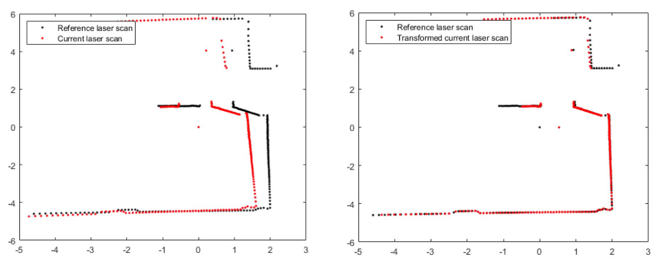
The Correspondence Problem

Key challenge: We usually don’t know which $p_i$ matches which $q_j$!

• Same physical point may not be observed in both scans
• Points have different indices in each scan
• Some points have no match at all

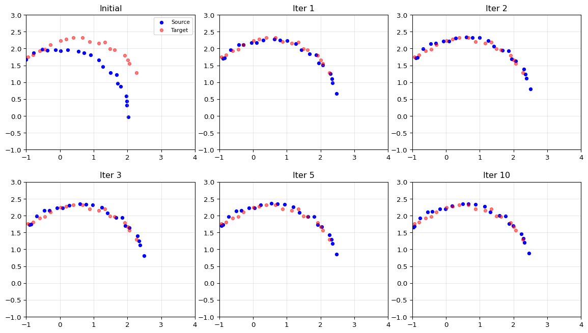
Solution: Iteratively estimate correspondences and transformation

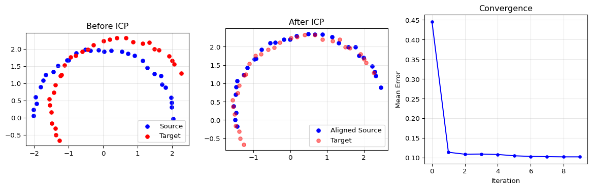
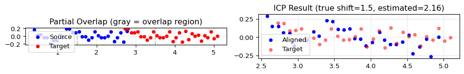
Part 2: The ICP Algorithm

Iterative Closest Point (ICP)

Core idea: Alternate between:

1. Finding correspondences: For each point, find its nearest neighbor
2. Solving for transformation: Given correspondences, find best $(R, \mathbf{t})$

Repeat until convergence

ICP Algorithm: Pseudocode

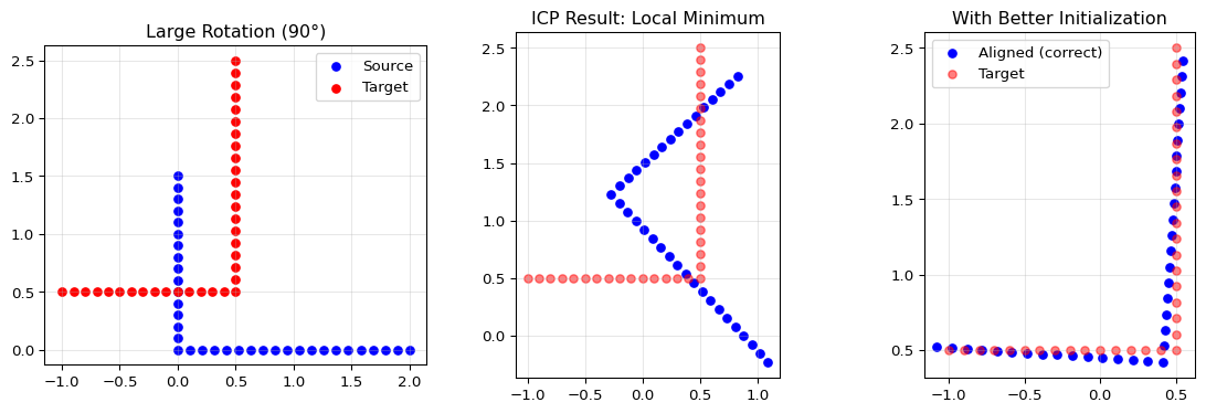
Input: Source points P, Target points Q, initial guess T₀
Output: Transformation T aligning P to Q

T ← T₀
repeat:
    P' ← apply T to P

    # Step 1: Find correspondences
    for each p' in P':
        c(p') ← nearest neighbor of p' in Q

    # Step 2: Compute optimal transformation
    T_new ← solve_alignment(P', correspondences)
    T ← T_new ∘ T

until convergence
return T

ICP Step 1: Nearest Neighbor

For each transformed source point $p'_i$, find: $$c(i) = \arg\min_j \| p'_i - q_j \|$$

Implementation:

• Brute force: $O(nm)$ for $n$ source, $m$ target points
• KD-tree: $O(n \log m)$ average case

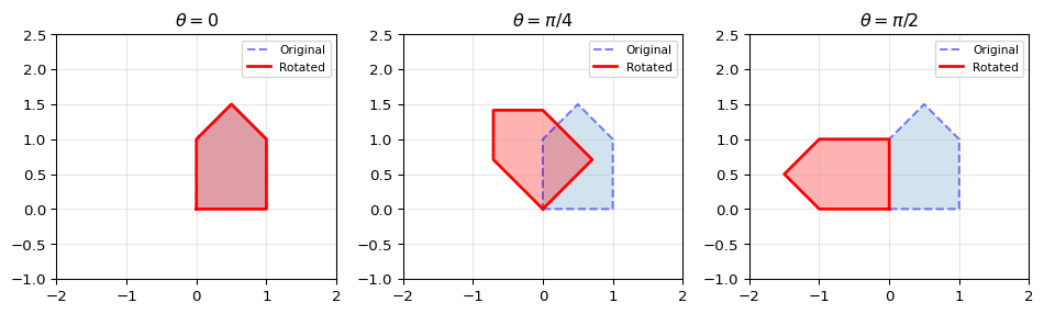
ICP Step 2: Solve for Transformation

Given correspondences, minimize: $$\sum_i \| R p_i + \mathbf{t} - q_{c(i)} \|^2$$

Closed-form solution (Arun et al., 1987):

1. Compute centroids: $\bar{p} = \frac{1}{n}\sum p_i$, $\bar{q} = \frac{1}{n}\sum q_{c(i)}$
2. Center the points: $p'_i = p_i - \bar{p}$, $q'_i = q_{c(i)} - \bar{q}$
3. Compute $H = \sum p'_i q'^T_i$
4. SVD: $H = U \Sigma V^T$, then $R = V U^T$
5. Translation: $\mathbf{t} = \bar{q} - R\bar{p}$

ICP Implementation

import numpy as np

def nearest_neighbors(source, target):
    """Find nearest neighbor in target for each source point."""
    indices = []
    for p in source.T:
        dists = np.linalg.norm(target.T - p, axis=1)
        indices.append(np.argmin(dists))
    return np.array(indices)

def compute_transformation(source, target_matched):
    """Compute optimal R, t using SVD."""
    # Centroids
    centroid_s = source.mean(axis=1, keepdims=True)
    centroid_t = target_matched.mean(axis=1, keepdims=True)
    # Center points
    s_centered = source - centroid_s
    t_centered = target_matched - centroid_t
    # SVD
    H = s_centered @ t_centered.T
    U, _, Vt = np.linalg.svd(H)
    R = Vt.T @ U.T
    # Ensure proper rotation (det = 1)
    if np.linalg.det(R) < 0:
        Vt[-1, :] *= -1
        R = Vt.T @ U.T
    t = centroid_t - R @ centroid_s
    return R, t.flatten()

ICP: Full Algorithm

def icp(source, target, max_iters=50, tol=1e-6):
    """
    Iterative Closest Point algorithm.
    source, target: 2×N arrays of 2D points
    Returns: R (2×2), t (2,), history of errors
    """
    R_total = np.eye(2)
    t_total = np.zeros(2)
    errors = []

    current = source.copy()
    for _ in range(max_iters):
        # Step 1: Find correspondences
        indices = nearest_neighbors(current, target)
        matched = target[:, indices]

        # Compute error
        error = np.mean(np.linalg.norm(current - matched, axis=0))
        errors.append(error)

        # Step 2: Compute transformation
        R, t = compute_transformation(current, matched)

        # Apply transformation
        current = R @ current + t.reshape(2, 1)

        # Accumulate
        R_total = R @ R_total
        t_total = R @ t_total + t

        # Check convergence
        if len(errors) > 1 and abs(errors[-2] - errors[-1]) < tol:
            break

    return R_total, t_total, errors

ICP Demo: Synthetic Data

np.random.seed(42)

# Generate source points (arc shape)
theta_pts = np.linspace(0, np.pi, 30)
source = np.vstack([2*np.cos(theta_pts), 2*np.sin(theta_pts)])
source += 0.05 * np.random.randn(*source.shape)  # Add noise

# Create target by applying known transformation
true_theta = np.pi / 6  # 30 degrees
true_t = np.array([0.5, 0.3])
R_true = rotation_matrix(true_theta)
target = R_true @ source + true_t.reshape(2, 1)

# Run ICP
R_est, t_est, errors = icp(source, target)

# Visualize
fig, axes = plt.subplots(1, 3, figsize=(12, 4))

# Before ICP
axes[0].scatter(source[0], source[1], c='blue', s=30, label='Source')
axes[0].scatter(target[0], target[1], c='red', s=30, label='Target')
axes[0].set_title('Before ICP'); axes[0].legend()
axes[0].set_aspect('equal'); axes[0].grid(True, alpha=0.3)

# After ICP
aligned = R_est @ source + t_est.reshape(2, 1)
axes[1].scatter(aligned[0], aligned[1], c='blue', s=30, label='Aligned Source')
axes[1].scatter(target[0], target[1], c='red', s=30, alpha=0.5, label='Target')
axes[1].set_title('After ICP'); axes[1].legend()
axes[1].set_aspect('equal'); axes[1].grid(True, alpha=0.3)

# Convergence
axes[2].plot(errors, 'b-o', markersize=4)
axes[2].set_xlabel('Iteration'); axes[2].set_ylabel('Mean Error')
axes[2].set_title('Convergence'); axes[2].grid(True, alpha=0.3)

plt.tight_layout()
plt.show()

print(f"True rotation: {np.degrees(true_theta):.1f}°, Estimated: {np.degrees(np.arctan2(R_est[1,0], R_est[0,0])):.1f}°")
print(f"True translation: {true_t}, Estimated: {t_est.round(3)}")

True rotation: 30.0°, Estimated: 16.3°
True translation: [0.5 0.3], Estimated: [0.505 0.35 ]

ICP Animation

# Show ICP iterations step by step
fig, axes = plt.subplots(2, 3, figsize=(12, 7))
axes = axes.flatten()

# Run ICP manually to capture intermediate states
current = source.copy()
R_acc, t_acc = np.eye(2), np.zeros(2)

iterations_to_show = [0, 1, 2, 3, 5, 10]
states = [(source.copy(), "Initial")]

for i in range(12):
    indices = nearest_neighbors(current, target)
    matched = target[:, indices]
    R, t = compute_transformation(current, matched)
    current = R @ current + t.reshape(2, 1)
    R_acc = R @ R_acc
    t_acc = R @ t_acc + t
    if i + 1 in iterations_to_show:
        states.append((current.copy(), f"Iter {i+1}"))

for ax, (pts, title) in zip(axes, states[:6]):
    ax.scatter(pts[0], pts[1], c='blue', s=20, label='Source')
    ax.scatter(target[0], target[1], c='red', s=20, alpha=0.5, label='Target')
    ax.set_title(title)
    ax.set_xlim(-1, 4); ax.set_ylim(-1, 3)
    ax.set_aspect('equal'); ax.grid(True, alpha=0.3)

axes[0].legend(fontsize=8)
plt.tight_layout()
plt.show()

Part 3: Practical Intuition

When ICP Works Well

ICP converges reliably when:

• Good initialization: Initial guess is close to true transformation
• Sufficient overlap: Most source points have valid matches in target
• Low noise: Point positions are accurate

Rule of thumb: Initial rotation error < 30-45° for typical data

Local Minima: The Main Failure Mode

np.random.seed(123)

# Create an L-shaped point cloud
L_shape = np.hstack([
    np.vstack([np.linspace(0, 2, 20), np.zeros(20)]),
    np.vstack([np.zeros(15), np.linspace(0.1, 1.5, 15)])
])

# Large rotation (90 degrees)
true_theta_large = np.pi / 2
R_large = rotation_matrix(true_theta_large)
target_large = R_large @ L_shape + np.array([[0.5], [0.5]])

# Run ICP with NO initialization
R_bad, t_bad, errors_bad = icp(L_shape, target_large)
aligned_bad = R_bad @ L_shape + t_bad.reshape(2, 1)

fig, axes = plt.subplots(1, 3, figsize=(12, 4))

# Problem setup
axes[0].scatter(L_shape[0], L_shape[1], c='blue', s=30, label='Source')
axes[0].scatter(target_large[0], target_large[1], c='red', s=30, label='Target')
axes[0].set_title('Large Rotation (90°)'); axes[0].legend()
axes[0].set_aspect('equal'); axes[0].grid(True, alpha=0.3)

# ICP result (likely wrong)
axes[1].scatter(aligned_bad[0], aligned_bad[1], c='blue', s=30, label='Aligned (wrong!)')
axes[1].scatter(target_large[0], target_large[1], c='red', s=30, alpha=0.5, label='Target')
axes[1].set_title('ICP Result: Local Minimum')
axes[1].set_aspect('equal'); axes[1].grid(True, alpha=0.3)

# With good initialization
R_init = rotation_matrix(np.pi/2 * 0.8)  # Start closer
source_init = R_init @ L_shape
R_good, t_good, errors_good = icp(source_init, target_large)
R_final = R_good @ R_init
aligned_good = R_final @ L_shape + t_good.reshape(2, 1)

axes[2].scatter(aligned_good[0], aligned_good[1], c='blue', s=30, label='Aligned (correct)')
axes[2].scatter(target_large[0], target_large[1], c='red', s=30, alpha=0.5, label='Target')
axes[2].set_title('With Better Initialization')
axes[2].set_aspect('equal'); axes[2].grid(True, alpha=0.3)
axes[2].legend()

plt.tight_layout()
plt.show()

Partial Overlap Problem

np.random.seed(456)

# Create a longer line
line = np.vstack([np.linspace(0, 4, 50), 0.1*np.random.randn(50)])

# Target is shifted version with partial overlap
shift = 1.5
target_partial = line[:, 15:45].copy()  # Only middle portion
target_partial[0] += shift

# Source is different portion
source_partial = line[:, 5:35].copy()

# Run ICP
R_p, t_p, err_p = icp(source_partial, target_partial)
aligned_p = R_p @ source_partial + t_p.reshape(2, 1)

fig, axes = plt.subplots(1, 2, figsize=(10, 4))

axes[0].scatter(source_partial[0], source_partial[1], c='blue', s=20, label='Source')
axes[0].scatter(target_partial[0], target_partial[1], c='red', s=20, label='Target')
axes[0].axvline(x=1.5, color='gray', linestyle='--', alpha=0.5)
axes[0].axvline(x=3.5, color='gray', linestyle='--', alpha=0.5)
axes[0].set_title('Partial Overlap (gray = overlap region)')
axes[0].legend(); axes[0].set_aspect('equal'); axes[0].grid(True, alpha=0.3)

axes[1].scatter(aligned_p[0], aligned_p[1], c='blue', s=20, label='Aligned')
axes[1].scatter(target_partial[0], target_partial[1], c='red', s=20, alpha=0.5, label='Target')
axes[1].set_title(f'ICP Result (true shift={shift}, estimated={t_p[0]:.2f})')
axes[1].legend(); axes[1].set_aspect('equal'); axes[1].grid(True, alpha=0.3)

plt.tight_layout()
plt.show()

Warning

Partial overlap causes ICP to underestimate translation!

What Can Go Wrong: Summary

Problem	Symptom	Mitigation
Large rotation	Converges to wrong pose	Better initialization
Partial overlap	Underestimated translation	Outlier rejection
Noise/outliers	Slow convergence, bias	Robust cost functions
Symmetric geometry	Multiple valid solutions	Additional constraints

Debugging Strategies

1. Test on synthetic data first

• Create target from known transformation of source
• You know the ground truth!

2. Visualize intermediate results

• Plot correspondences at each iteration
• Check if matches make geometric sense

3. Monitor convergence

• Error should decrease monotonically
• Sudden jumps indicate problems

Numerical Gradient Check

Verify your Jacobian by comparing to finite differences:

def numerical_gradient(f, x, eps=1e-5):
    """Compute gradient numerically using central differences."""
    grad = np.zeros_like(x)
    for i in range(len(x)):
        x_plus = x.copy(); x_plus[i] += eps
        x_minus = x.copy(); x_minus[i] -= eps
        grad[i] = (f(x_plus) - f(x_minus)) / (2 * eps)
    return grad

# Example: cost function for alignment
def alignment_cost(params, source, target_matched):
    theta, tx, ty = params
    R = rotation_matrix(theta)
    transformed = R @ source + np.array([[tx], [ty]])
    return np.sum((transformed - target_matched)**2)

# Test
params = np.array([0.1, 0.2, 0.3])
grad = numerical_gradient(lambda p: alignment_cost(p, source[:,:5], target[:,:5]), params)
print(f"Numerical gradient: {grad.round(4)}")

Numerical gradient: [-14.9754   1.2598  -7.2557]

Assignment 1

Project Goal

Goal

The goal of the assignment is to generate an image depicting a map of the environment in which a sequence of 2D LiDAR scans were recorded.

Your team must create code that

• saves the map in a .png file,
• save the poses associated with every scan in the provided list of scans, assuming the first scan is at $(0,0,0)$, in a .npz file.

Example

Robot Pose

The pose of the robot in a world frame is described by three numbers:

$$(X_i, Y_i, \theta_i)$$

• $(X_i, Y_i)$: Position of robot (origin of robot frame) in world frame
• $\theta_i$: Orientation angle (direction where $\phi = 0$ points)

When robot frame coincides with world frame: pose is $(0, 0, 0)$

Coordinate Transformation

Given scan points $\left\{(x_j, y_j)\right\}$ in the robot frame at pose $(\Delta X_i, \Delta Y_i, \Delta \theta_i)$ relative to the current frame $F$:

$$\begin{aligned} x_{F} &= \Delta X_i + x_j \cos \Delta \theta_i - y_j \sin \Delta \theta_i \\ y_{F} &= \Delta Y_i + x_j \sin \Delta \theta_i + y_j \cos \Delta \theta_i \end{aligned}$$

Relative pose transforms all points in the robot frame to the frame $F$

Scan Matching as Optimization

To match two scans:

1. Treat one scan as the reference frame
2. Find $(\Delta X_i, \Delta Y_i, \Delta \theta_i)$ that transforms the second scan to align with the reference

Goal: Find the transformation that provides the best alignment

Instructions

• Teams of up to two individuals
• Input: 2D laser scans in sims_N_scans.npz or .mat
• Output:
  • Sequence of poses $(X_i, Y_i, \theta_i)$ (.npz file)
  • Estimated map of the environment in which scans were taken (.png file)

Evaluation Criteria

The evaluation is based on

• Sum of squared errors between true and estimated relative poses between temporally successive poses.
• Relative error in the final position and orientation relative to ground truth.

Hints

• You can use scan matching to get an estimate of where the robot was at different times
  • Chain the relative transformations
  • Accumulate poses in the world frame
• You can then use pose graph optimization to correct the drift over time using long-range connections, by defining a suitable set of edges
• Two popular methods for scan matching involve the Iterative Closes Point algorithm, and the Normal Distribution Transform
  • Copying from existing implementations of these algorithms that produce highly accurate predictions is not success

Testing Strategy

Test on synthetic ideal data where you know the answer:

Pure translation test: $$(x'_i, y'_i) = (x_i + \Delta x^*, y_i)$$

Pure rotation test: $$(x'_i, y'_i) = (x_i \cos \theta^* - y_i \sin \theta^*, x_i \sin \theta^* + y_i \cos \theta^*)$$

For synthetic data: same point appears in both scans, so use direct point-to-point error

Summary

1. Rigid transformations: $R(\theta)$ and SE(2) describe 2D motion
2. Point cloud alignment: Minimize sum of squared residuals
3. ICP algorithm: Iterate between correspondence and transformation
4. Local minima: ICP needs good initialization