ME/AER 647 Systems Optimization I

---

Line Search

Instructor: Hasan A. Poonawala

Mechanical and Aerospace Engineering
University of Kentucky, Lexington, KY, USA

Topics:
Wolfe Conditions
Backtracking Line Search
Convergence properties

Step size selection

Recap

• In Unconstrained Optimization we saw theory that suggests algorithms:
  • In proof of First Order Necessary Conditions, we saw that choosing $p_k = -\nabla f_k$ and $\alpha_k$ implies $f(x_{k+1}) < f(x_k)$
    • However, decreasing $f_k$ does not imply we reach the optimum if the decrease is too small
  • Another strategy from the Sufficient Conditions is to solve $\|\nabla f(x) = 0\|$
• Now we look at rules for $\alpha_k$ and $p_k$ in an algorithm $x_{k+1} = x_k + \alpha_k p_k$ that will
  • decrease $f(x_k)$ enough so that
  • we solve $\|\nabla f(x) = 0\|$

Lipschitz Function

A function $f \colon \mathbb{R}^m \to \mathbb{R}$ is Lipschitz on a set $S$ if for any $x,y \in S$ $$\|f(x) - f(y) \| \leq L \|x - y\|$$

For twice differentiable functions, $\nabla f$ being differentiable is equivalent to $$\nabla^2 f(w) \preceq L I$$ for all $w \in S$

Steepest Descent

Descent Lemma

Let $f$ be a twice differentiable function whose gradient $\nabla f$ is Lipschitz continuous over some convex set $S$. Then, for all $x,y \in S$, by Taylor’s Theorem, $$f(y) = f(x) + \nabla f(x)^T (y-x) + \frac{1}{2} (y-x)^T \nabla^2 f(z) (y-x)$$

$$\implies f(y) \leq f(x) + \nabla f(x)^T (y-x) + \frac{L}{2} \|y-x\|^2,$$

This Lemma says that we can define a local quadratic function that is an upper bound for $f$ near a point $x$.

If $x = x_k$ and $y = x_k - \alpha_k \nabla f_k$, we get $$f_{k+1} \leq f_k -\frac{\alpha_{k} (2 - L \alpha_{k} )}{2} \|\nabla f_k\|^2$$

• If $0 < \alpha_k < \frac{2}{L}$, then $f_{k+1} < f_{k}$.
• $f_{k}-f_{k+1}$ approaches zero only when $\nabla f_k \to 0$

Example

$$min_{x \in \mathbb{R}} \quad f(x) = (x-3)^2$$

$$\nabla^2 f = 2$$

To ensure decrease, we need $$\alpha < \frac{2}{L} = 1$$

If $\alpha =1$, then $f_{k+1} = f_{k}$

If $x_k = x^{\star} + y$, then $x_{k+1} = x^{\star} -y$

Optimal Steepest Descent

Descent Lemma: $$f_{k+1} \leq f_k -\frac{\alpha_{k} (2 - L \alpha_{k} )}{2} \|\nabla f_k\|^2$$

The smallest bound on $f_{k+1}$ occurs when $\alpha_k = 1/L$: $$f_{k+1} \leq f_k -\frac{1}{2 L} \|\nabla f_k\|^2$$

But what happens when we don’t know $L$?

• Start with small $\hat L$, check whether $f_{k+1} \leq f_k -\frac{1}{2 \hat L} \|\nabla f_k\|^2$
• If not satisfied, double $\hat L$, repeat

This is a preview of backtracking

Wolfe Conditions

• Sufficient decrease condition (Armijo rule) on $\alpha_k$: $$f(x_k + \alpha_k p_k) \leq f(x_k) + c_1 \alpha_k \nabla f(x_k)^T p_k$$
• Curvature condition on $\alpha_k$: $$\nabla f(x_k + \alpha_k p_k)^T p_k \geq c_2 \nabla f(x_k )^T p_k$$ with $0<c_1 < c_2 <1$.

• The sufficient condition prevents large steps that don’t provide enough benefit
  • Through a function that linearly links decrease in $f$ with size of $\alpha_k$
• The curvature condition prevents small steps that don’t provide enough benefit
  • Through a sufficient change in $\nabla f$

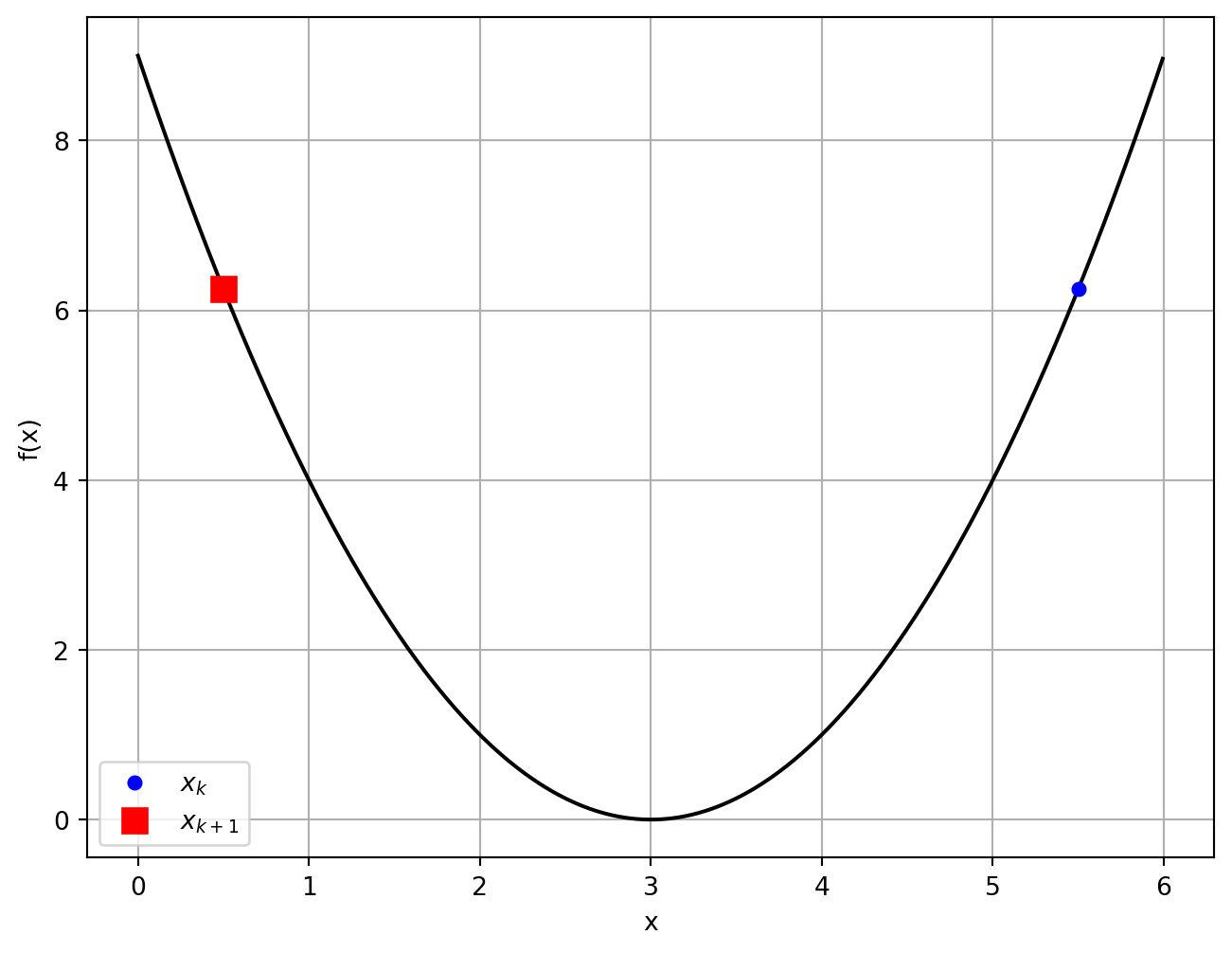
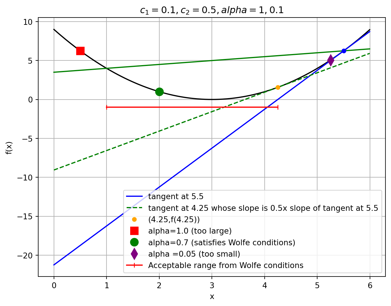
Example Wolfe Conditions

$$min_{x \in \mathbb{R}} f(x) = (x-3)^2$$

Backtracking

Replaces curvature condition with a reducing sequence of $\alpha$.

• Choose $\bar \alpha > 0, c \in (0,1) ,\rho \in (0,1)$
• Initialize $\alpha \gets \bar \alpha$    (start with large step)
• While $f(x_k + \alpha p_k) > f(x_k) + c \alpha \nabla f(x_k)^T p_k$
  • $\alpha = \rho \alpha$ (reduce if too large)

Example values: $\bar \alpha=1.0$, $c = 0.1$, $\rho = 0.5$

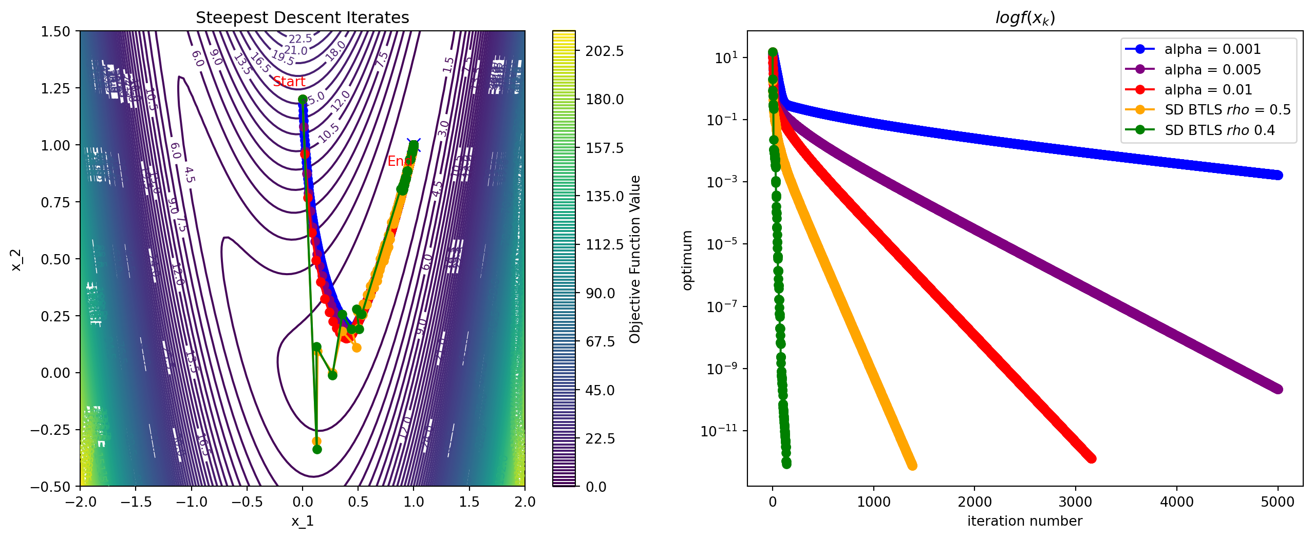
Backtracking Example

$$f(x) = (x-3)^2$$

Convergence Analysis

Convergence

Informally

Will $x_k \to x^{\star}?$

Weaker

Will $f(x_k) \to f(x^{\star})?$

Still weaker

Will $\|\nabla f(x_k) \|\to 0?$

Zoutendijk Condition

• Involves the angle between steepest descent direction and chosen direction $p_k$: $$\cos \theta_k = \frac{- \nabla f_k^T p_k}{\| \nabla f_k \| \|p_k\|}$$
• If $p_k = - \nabla f_k$, then $\cos \theta_k = 1$ and $\theta_k =0$
• If $\theta_k$ is $\pm 89^{\circ}$, then $\cos \theta_k > 0$ but small
• If $|\theta_k| \geq 90^{\circ}$, then $\cos \theta_k \leq 0$, and $p_k$ is not a strict descent direction

Theorem

Consider any iteration of the form $x_{k+1} =x_k + \alpha_k p_k$, where $p_k$ is a descent direction and $\alpha_k$ satisfies the Wolfe conditions. Suppose that $f$ is bounded below in $\mathbb{R}^n$ and that $f$ is continuously differentiable in an open set $\mathcal N$ containing the level set $\mathcal L = \{x \colon f(x) \leq f(x_0)\}$. Assume also that the gradient $\nabla f$ is Lipschitz continuous on $\mathcal N$, then $$\sum_{k=0}^{\infty} \cos^2 \theta_k \|\nabla f_k \|^2 < \infty$$

Convergence from Zoutendijk Condition

If we choose $p_k$ such that $\cos \theta_k \geq \delta >0$ for all $k \geq 0$, then the Zoutendijk condition implies that $$\lim_{k \to \infty} \|\nabla f_k \| = 0$$

• If $B_k$ is positive definite with uniformly bounded condition number ($\| B_k \| \|B_k^{-1}\| \leq M < \infty$), then for $p_k =-B_k^{-1}\nabla f_k$, $$\cos \theta_k \geq \frac{1}{M}$$
  • What algorithm does this conclusion apply to when $B_k = I$ or $B_k = \nabla^2 f \succ 0$?

Similar results apply to $\alpha_k$ chosen using backtracking line search.

Convergence Rate

Informally

How fast does $x_k \to x^{\star}?$

Less informally

The convergence rate measures how fast the error in the solution decreases. The error can be in terms of the optimum $\|x_k - x^\star\|$, the optimal value $|f(x_k) - f(x^\star)|$, or $\|\nabla f(x_k)\|$.

Example

If $\|x_{k+1} - x^\star\| \leq \rho \|x_{k} - x^\star\|$ for constant $\rho <1$, then the convergence is linear. Moreover, the number of iterations $k = \mathcal O (\log \frac{1}{\epsilon})$.

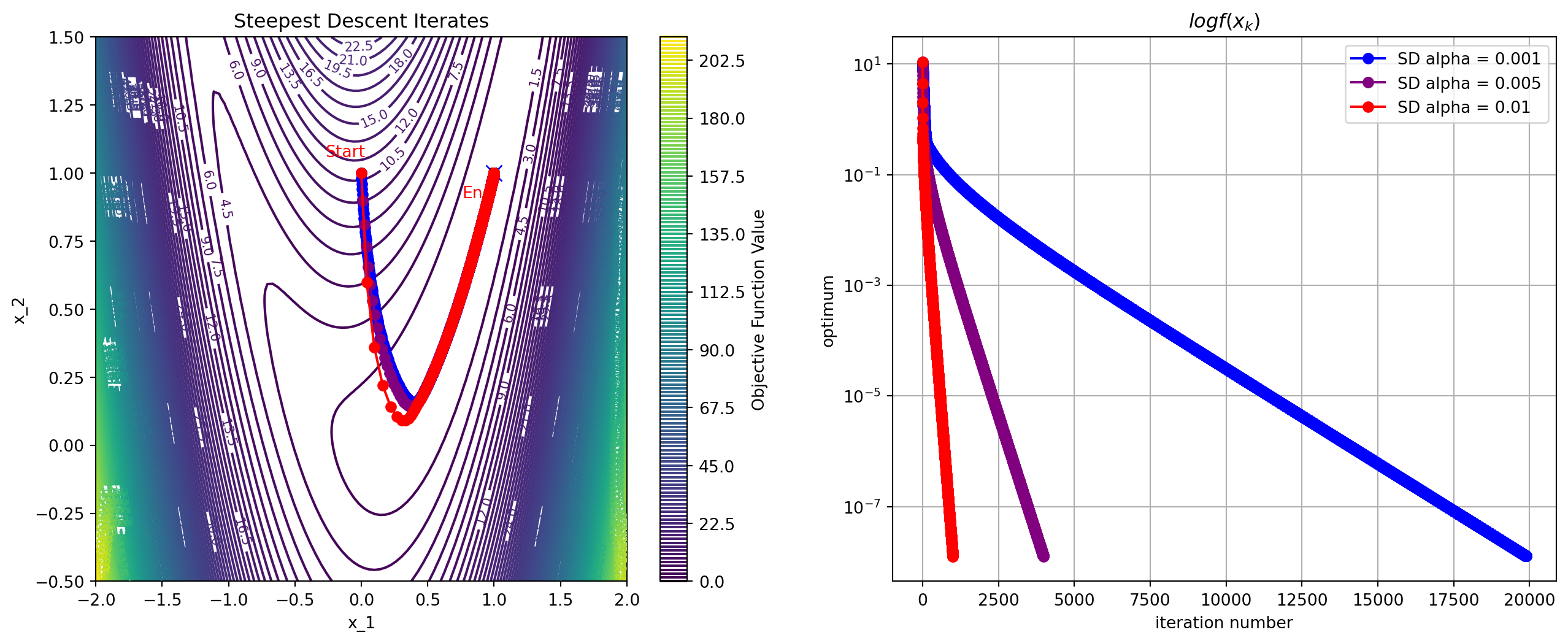
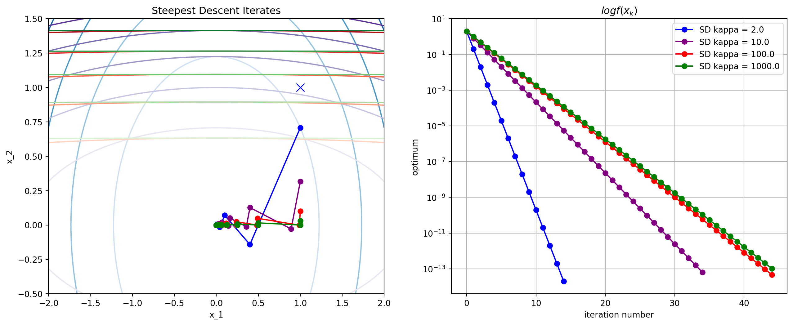
Convergence Rate of Steepest Descent with Exact Line Search

• When $f = x^T Q x - b^T x$ where $Q = Q^T \succ 0$, we get linear convergence in $\|x_k - x^\star\|$
  • See Theorem 3.3: $\| x_{k+1} - x^{\star} \|_Q \leq \rho \| x_{k} - x^{\star} \|_Q$, $\rho = \frac{ \frac{\lambda_{\max}(Q)}{\lambda_{\min}(Q)} -1} {\frac{\lambda_{\max}(Q)}{\lambda_{\min}(Q)} +1}$
  • If condition number is $800$, with $f(x_1)=1$ and $f(x^{\star})=0$, after 1000 iterations, objective is only $0.08$
• When $f$ is twice continuously differentiable, if $x^k \to x^\star$ where $x^\star$ satisfies SOSC, then we get linear convergence in $|f_k - f(x^\star)|$
  • See Theorem 3.4
• If we use inexact line search, the convergence is even slower

Rosenbrock Function

$$\log \epsilon = -m\ k + c \iff k = - \frac{1}{m} \log \epsilon -\frac{c}{m} \iff k = \frac{1}{m} \log \frac{1}{\epsilon} \quad + \frac{c}{m}$$

Condition Number

$$f(x,y) = x^2 + \kappa y^2$$

Newton’s Method

Motivation

• We know that whatever point we are looking must be a stationary one, it must satisfy $\nabla f(x) = 0$.

• Newton’s method applies the Newton root-finding algorithm to $\nabla f$:

  • To solve $g(x) = 0$, iteratively solve ¹ $$g(x_k) + (x_{k+1} - x_k)^T \nabla g(x) = 0 \implies x_{k+1} = x_k - (\nabla g(x) )^{\sharp} g(x)$$

• Apply root finding to $\nabla f(x) = 0$: $$x_{k+1} = x_k - (\nabla^2 f(x) )^{-1} \nabla f(x)$$

1. $\sharp$ is the left pseudo-inverse: $A^\sharp = (A^T A)^{-1} A^T$

Example

• We want to find the minimizer of

$$f(x) = \frac{1}{2}x^2 - \sin{x}, \quad x_0 = \frac{1}{2}.$$

• We want an accuracy of $\varepsilon = 10^{-5}$, i.e., stop when

$$|x_{k+1} - x_k | < \varepsilon.$$

• We compute

$$f'(x) = x - \cos{x}, \quad f''(x) = 1 + \sin{x}.$$

$$\begin{align} x_1 &= \frac{1}{2} - \frac{\frac{1}{2} - \cos{\frac{1}{2}}}{1 + \sin{\frac{1}{2}}} = 0.7552, \\ x_2 &= x_1 - \frac{f'(x_1)}{f''(x_1)} = x_1 - \frac{0.02710}{1.685} = 0.7391, \\ x_3 &= x_2 - \frac{f'(x_2)}{f''(x_2)} = x_2 - \frac{9.461 \times 10^{-5}}{1.673} = 0.7390, \\ x_4 &= x_3 - \frac{f'(x_3)}{f''(x_3)} = x_3 - \frac{1.17 \times 10^{-9}}{1.673} = 0.7390. \end{align}$$

Alternate Motivation

When $\nabla^2 f_k \succ 0$, we are minimizing the quadratic approximation $$f(x) \approx f_k + \nabla f_k^T (x-x_k) + \frac{1}{2} (x-x_k)^T \nabla^2 f_k (x-x_k),$$ which need not have minimum at $x^\star$

Example: Quadratic Function

Consider $$f(x) = x^T Q x - b^T x \quad \text{ for }Q=Q^T \succ 0,$$ where $x^\star = Q^{-1} b$ $$\begin{align} \text{ Ideal update: }&& x_{k+1} &= x_k - (x_k - x^\star) = x_k - 1 \cdot (x_k - Q^{-1} b )\\ \text{Newton update:}&& x_{k+1} &= x_k + 1 \cdot (-1) \cdot Q^{-1} (Q x_k - b) = x_k -1 \cdot (x_k - Q^{-1} b)\\ \text{Steepest descent:}&& x_{k+1} &= x_k + \alpha_k \cdot (-1) \cdot (Q x_k - b) \end{align}$$

What happens when $Q = Q^T \prec 0$?

Example: Rosenbrock Function

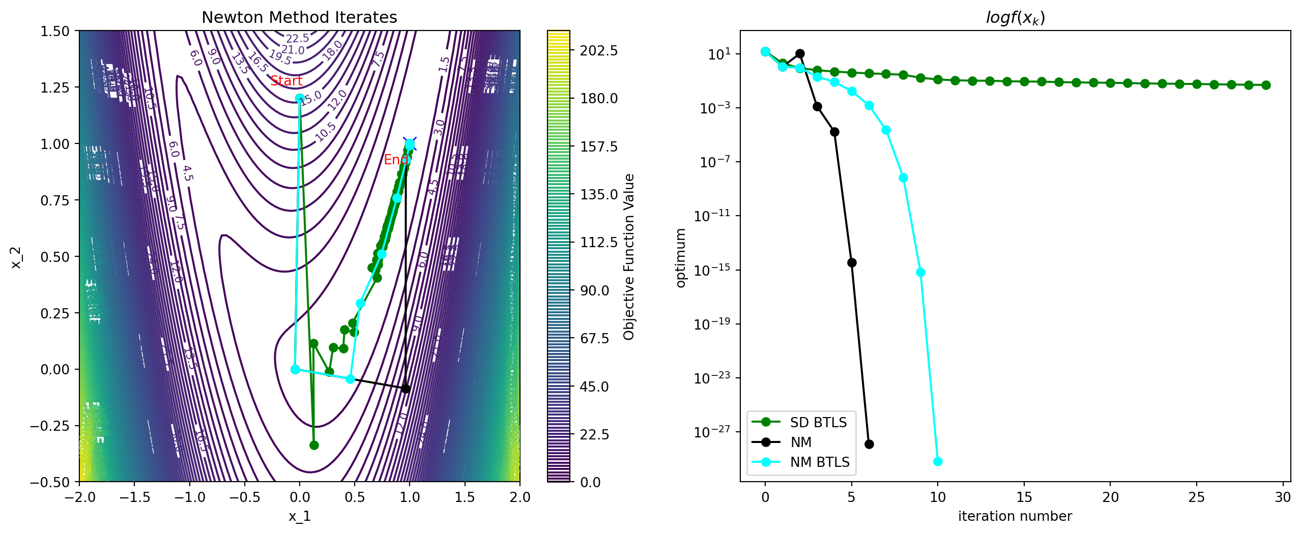
Convergence Rate

Theorem 3.5

Suppose that $f$ is twice differentiable and that the Hessian $\nabla^2 f$ is Lipschitz continuous in a neighborhood of a solution $x^\star$ at which the sufficient conditions are satisfied. Consider the iteration $x_{k+1} = x_k + p_k$ where $p_k = - \nabla^2 f_k^{-1} \nabla f_k$. Then

• If $x_0$ is sufficiently close to $x^\star$, then $x_k \to x^\star$
• The rate of convergence $\{x_k\}$ is quadratic
• The sequence of gradient norms $\{\|\nabla f_k\|\}$ converges quadratically to zero

Proof Outline

Here, we directly look at $\| x_{k + 1} - x^{\star}\|$, using $\nabla f\left( x^{\star} \right) = 0$

$$\begin{aligned} x_{k + 1} - x^{\star} & = x_{k} - \nabla^{2}f_{k}^{- 1}\nabla f_{k} - x^{\star} \\ & = \nabla^{2}f_{k}^{- 1}\left( \nabla^{2}f_{k}\left( x_{k} - x^{\star} \right) - \left( \nabla f_{k} - \nabla f\left( x^{\star} \right) \right) \right) \end{aligned}$$

Under the assumption that $\nabla^{2}f$ is $L$-Lipschitz, using Taylor’s theorem, we have $$\|\nabla^{2}f_{k}\left( x_{k} - x^{\star} \right) - \left( \nabla f_{k} - \nabla f\left( x^{\star} \right) \right)\| \leq \| x_{k} - x^{\star}\|^{2}\int_{0}^{1}Ltdt$$

For $\| x_{k} - x^{\star}\| \leq r$, we can rewrite this expression using

$$\| x_{k + 1} - x^{\star}\| \leq \|\nabla^{2}f_{k}^{- 1}\|\frac{L}{2}\| x_{k} - x^{\star}\|^{2}$$

For $\| x_{k} - x^{\star}\| \leq r$, we can rewrite this expression using $\overset{\sim}{L} = L\|\nabla^{2}f^{( - 1)}\left( x^{\star} \right)\|$ as

$$\| x_{k + 1} - x^{\star}\| \leq \overset{\sim}{L}\| x_{k} - x^{\star}\|^{2}$$

If $\|x_0 - x^\star\| < \min\left(r, \frac{1}{ \tilde{L}} \right)$, then we get quadratic convergence.

Newton’s Revenge

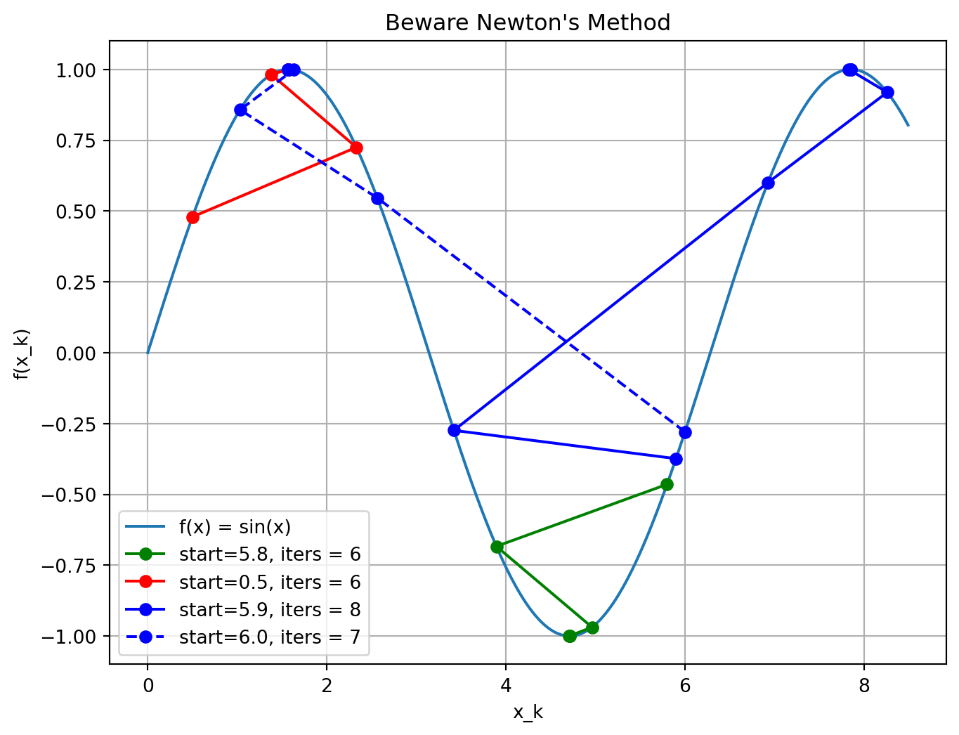
Modifications

Although Newton’s method is very attractive in terms of its convergence properties the solution, it requires modification before it can be used at points that are far from the solution.

The following modifications are typically used:

• Step-size reduction (damping)
• Modifying Hessian to be positive definite
• Approximation of Hessian

Damping

A search parameter $\alpha$ is introduced $$\bm{x}_{k+1} = \bm{x}_k - \alpha_k \nabla^2 f(\bm{x}_k)^{-1}\nabla f(\bm{x}_k),$$ where $\alpha_k$ is selected to minimize $f$.

A popular selection method is backtracking line search.

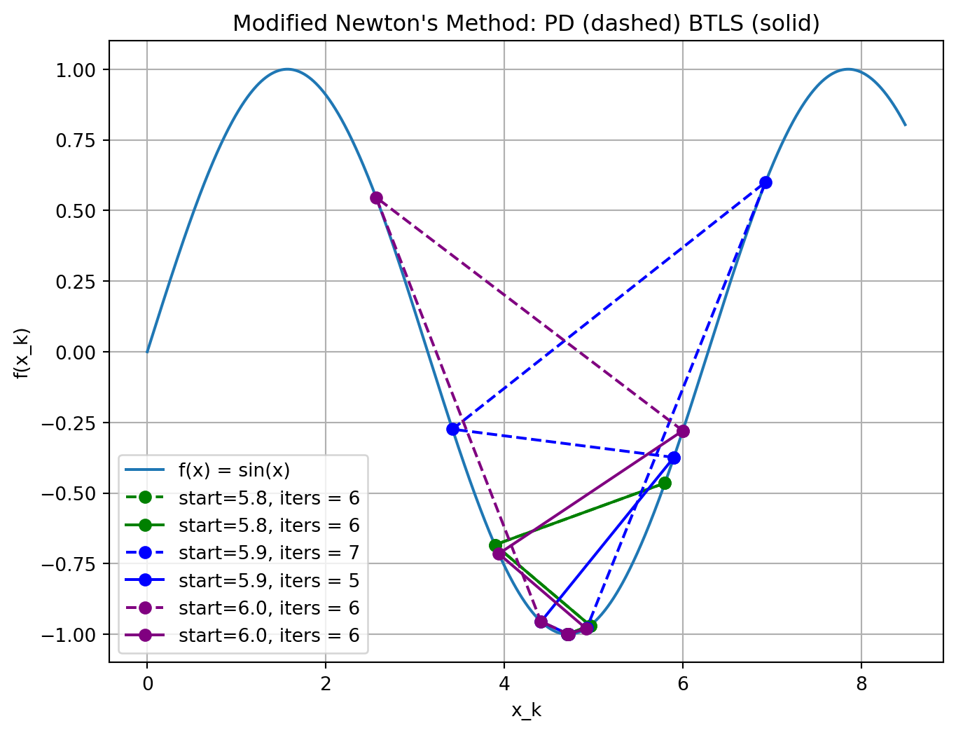
Positive Definiteness and Scaling

General class of algorithms is given by $$\bm{x}_{k+1} = \bm{x}_k + \alpha p_k = \bm{x}_k - \alpha B_k \nabla f_k, \qquad(1)$$

• SD: $B_k = \bm{I}$, Newton: $B_k = \nabla^2 f(\bm{x}_k)^{-1}$.

For small $\alpha$, it can be shown that $$f(\bm{x}_{k+1}) = f(\bm{x}_k) - \alpha \nabla f_k^T B_k \nabla f_k + O(\alpha^2).$$

• As $\alpha \rightarrow 0$, the second term on the rhs dominates the third.
• To guarantee a decrease in $f$, we must have $\nabla f_k^T B_k \nabla f_k > 0$.
  • Simplest way to ensure this is to require $B_k \succ \bm{0}$.

Positive Definiteness and Scaling

• In practice, Newton’s method must be modified to accommodate the possible non-positive definiteness of $\nabla^2 f$ at regions far from the solution.

• Common approach: $B_k = [\mu_k\bm{I} + \nabla^2 f(\bm{x}_k)]^{-1}$ for some $\mu_k > 0$.

• This can be regarded as a compromise between SD ($\mu_k$ very large) and Newton’s method ($\mu_k = 0$).

Levenberg-Marquardt performs Cholesky factorization for a given value of $\mu_k$ as follows $$\mu_k \bm{I} + \nabla^2 f(\bm{x}_k) = \bm{G}^T\bm{G}.$$

• This factorization checks implicitly for positive definiteness.

• If the factorization fails (matrix not PD) $\mu_k$ is increased.

• Step direction is found by solving $\bm{G}^T\bm{G} p_k = -\nabla f_k$.

Newton’s Revenge Avenged

Quasi-Newton Method

Computes $B_k \approx \nabla^2 f_k$ as a solution to the secant equation: $$B_{k+1} \underbrace{(x_{k+1}-x_{k})}_{s_k} = \underbrace{\nabla f_{k+1}-\nabla f_k}_{y_k}$$

Then solve $p_{k} = - B_k^{-1} s_{k}$

One dimension

$\frac{\partial^2 f}{\partial x^2} \approx \frac{\frac{\partial}{\partial x} f(x_{k+1}) - \frac{\partial}{\partial x} f(x_k)}{x_{k+1} -x_{k}}$

Quasi-Newton Method

Algorithms for updating $B_k$:

1. Broyden, Fletcher, Goldfarb, and Shanno (BFGS): $$B_{k+1} = B_{k} - \frac{B_{k}s_{k}s_{k}^TB_{k}}{s_{k}^TB_{k}s_k} + \frac{y_k y_k^T}{y_k^T s_k}$$

2. Symmetric Rank-One (SR1): $$B_{k+1} = B_{k} + \frac{(y_{k}-B_{k} s_{k})(y_{k}-B_{k} s_{k})^T}{(y_{k}-B_{k} s_{k})^Ts_{k}}$$

Algorithms for updating $H_k = B_k^{-1}$:

$$H_{k+1} = ( I - \rho_k s_k y_k^T) H_k ( I - \rho_k y_k s_k^T) + \rho_k s_k s_k^T, \quad \rho_k = \frac{1}{y_k^T s_k}$$ $$p_k = - H_k \nabla f_k$$

Quasi-Newton Method: Details

• Initialization: Start with $H_k = I$

• Step size: $\alpha_k = 1$ for all $k$ may interfere with $H_k$ approximating the Hessian

  • Backtracking isn’t enough to choose good $\alpha_k$
  • Choose $\alpha_k$ to satisfy strong Wolfe conditions
  • Details are very technical (numerical computing challenges)

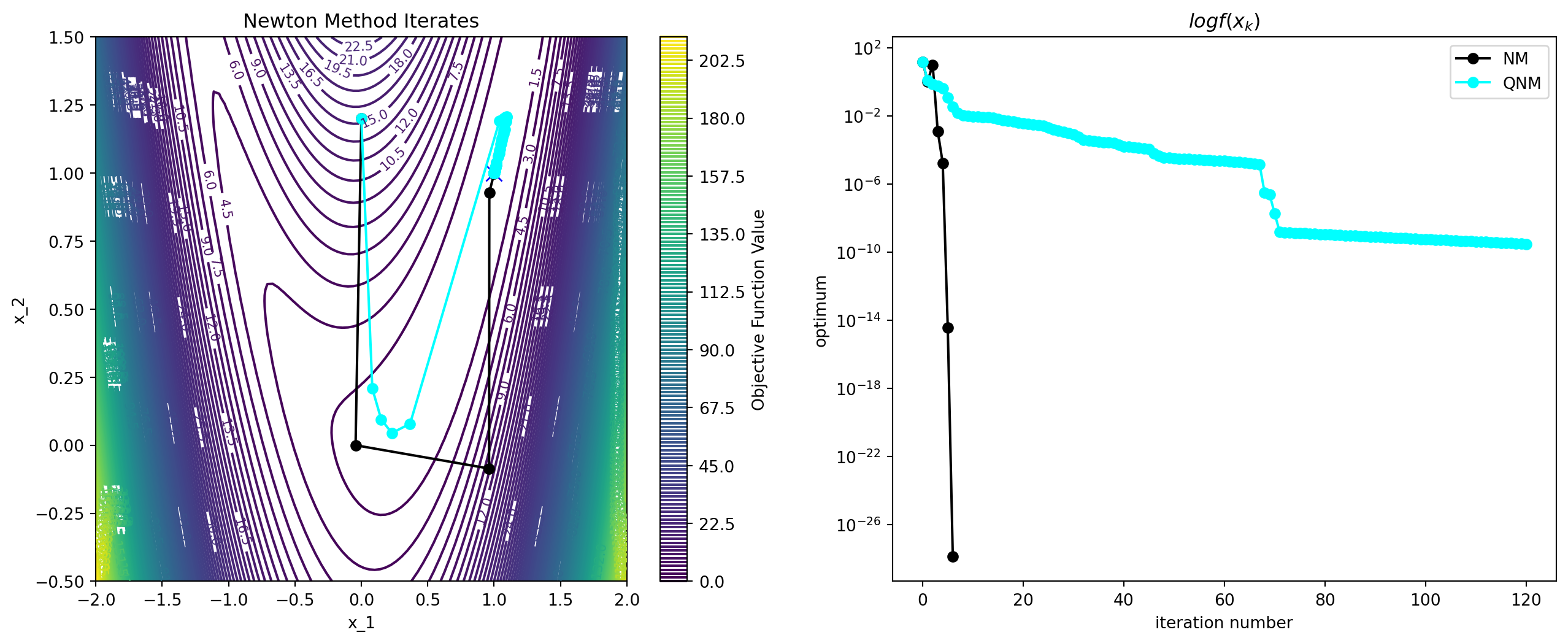
Example: Rosenbrock Function

Summary

Summary

You can now minimize $f(x)$ (when unconstrained) iteratively. Find LM $x^\star$ by

• Choosing direction $p_k$
  • Steepest descent with constant step size is easy and reliable but slow
  • Newton method is fast but expensive and unreliable
    • needs modifications for reliable convergence
  • Quasi-newton methods are a balance, but tricky
• Choosing step size $\alpha_k$
  • Back-tracking for SD and modified NM improves performance
  • Strong Wolfe conditions for Quasi-newton methods
• Not tackled: constraints, expensive $f$/$\nabla f$, discrete $x$, non-smooth $f$