PyTorch

Introduction

PyTorch, accessed via the torch package, is a scientific computing framework centered on representing data as tensors and automatic differentiation of tensor operations, making it easy to implement differentiable computing. Deep learning is one of its most popular applications, where differentiation of loss functions to form gradients is key to training models on data.

Tensors

Tensors in torch are \(n\)-dimensional array objects, similar to numpy arrays. In fact, you can easily switch:

import numpy as np
import torch

a = np.array([1.0, 2.0])
b = torch.from_numpy(a)           # NumPy → PyTorch (shares memory!)
c = b.numpy()                     # PyTorch → NumPy (also shares memory!)

However, torch tensor objects contain additional information and methods related to automatic differentiation and where it is located in system memory.

Autograd

Deep learning is nearly impossible without the ability to automatically differentiate models. Before that, demonstrating the value of a new model required careful derivation and implementation of its gradients. Now, all of that work has been automated away.

import torch

t = torch.Tensor([0.8762])
print(t) # This variable is not considered for gradient computations
t.requires_grad = True 
print(t) # Now it is
torch.sigmoid(t).backward() # calculate gradient (of sigmoid(t))
manual_grad = torch.sigmoid(t) * (1 - torch.sigmoid(t)) # manually calculated gradient of sigmoid
print("torch grad: ", t.grad.item()," manual gradient: ", manual_grad.item())

tensor([0.8762])
tensor([0.8762], requires_grad=True)
torch grad:  0.20754991471767426  manual gradient:  0.20754991471767426

Note that \(\sigma(x) = \frac{1}{1+e^{-x}}\) has derivative \(\sigma'(x) = \frac{e^{-x}}{(1+e^{-x})^2} = \sigma(x) (1-\sigma(x))\)

Turning off gradient tracking

PyTorch must do extra work to track gradients. This work will be done whenever we call the model, which is wasteful when we are calling it to perform inference using the trained model. To tell PyTorch we won’t need gradients, the inference is performed using the no_grad() method:

model.eval()    # tell pytorch that we will use the model in evaluation mode
with torch.no_grad(): # don't track gradients 
    outputs = model(X_test) # make predictions on the test set

Application: Linear Model

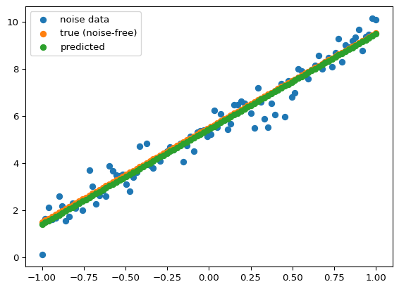
We fit a linear model to scalar input-output data in the simple models lesson using gradient descent ‘by hand’. Here, we use PyTorch. There are two differences from the pattern we saw at the end of the lesson on simple models:

The model is defined separately from the loss.
We don’t implement a gradient function, autodiff will derive it for us.

## Plot iterates and loss under GD using torch
## Train a linear model using pytorch

import torch
import torch.nn as nn
import torch.optim as optim
import numpy as np
import matplotlib.pyplot as plt

# 1. Create data
## First as numpy array
x = np.linspace(-1,1,100) 
y_noise_free = 4*x + 5
y = y_noise_free+0.5*np.random.randn(100)


## Create tensors, as 2D arrays using unsqueeze 
X_train = torch.tensor(x, dtype=torch.float32).unsqueeze(1)
y_train = torch.tensor(y, dtype=torch.float32).unsqueeze(1)

print(X_train.shape) ## two dimensions now
print(y_train.shape)


# 2. Define Linear model
class Lin(nn.Module):
    def __init__(self):
        super().__init__()
        self.net =  nn.Linear(1, 1)

    def forward(self, x):
        return self.net(x)
model = Lin()

# 3. Define loss 
criterion = nn.MSELoss() # Mean Squared Error

print("Start training: ")
# 4. Training loop
for epoch in range(5000):
    model.train()       # Tell pytorch that model computations are for training now
    model.zero_grad()   # clear accumulated grads
    outputs = model(X_train) # predict values ... 
    loss = criterion(outputs, y_train) # ... so we can compute loss 
    loss.backward()     # Automatically get gradients of loss wrt model as it is right now
    with torch.no_grad(): ## Manually implementing gradient descent. Don't want the update to be tracked by autograd
        for param in model.parameters():
            param -= 0.005 * param.grad  # θ ← θ − α∇θ L

    if (epoch + 1) % 500 == 0: ## Show us the loss as training proceeds
        print(f"Epoch {epoch+1}/5000 - Loss: {loss.item():.4f}")

# 5. Evaluation
model.eval()    # tell pytorch that we will use the model in evaluation mode
with torch.no_grad():
    outputs = model(X_train).numpy() # convert predictions to numpy array to work with matplotlib
    plt.scatter(x,y,label="noise data")
    plt.scatter(x,y_noise_free,label="true (noise-free)")
    plt.scatter(x,outputs[:,0],label="predicted")
    plt.legend()

torch.Size([100, 1])
torch.Size([100, 1])
Start training: 
Epoch 500/5000 - Loss: 0.4889
Epoch 1000/5000 - Loss: 0.2364
Epoch 1500/5000 - Loss: 0.2281
Epoch 2000/5000 - Loss: 0.2278
Epoch 2500/5000 - Loss: 0.2278
Epoch 3000/5000 - Loss: 0.2278
Epoch 3500/5000 - Loss: 0.2278
Epoch 4000/5000 - Loss: 0.2278
Epoch 4500/5000 - Loss: 0.2278
Epoch 5000/5000 - Loss: 0.2278